Data Structures & Types

CS&SS 508 • Lecture 6

Jess Kunke (slides adapted from Victoria Sass)

Roadmap

Last time, we learned:

• Importing and Exporting Data
• Tidying and Reshaping Data
• Types of Data
  • Wrangling Date/Date-Time Data

Today, we will cover:

• Types of Data
  • Factors
  • Numbers
  • Missing Values
• Data Structures
  • Vectors
  • Matrices
  • Lists

This week we start getting more into the weeds of programming in R.

These skills will help you understand some of R’s quirks, how to troubleshoot errors when they arise, and how to write more efficient and automated code that does a lot of work for you!

Data types in R

Returning, once again, to our list of data types in R:

• Logicals
• Factors
• Date/Date-time
• Numbers
• Missing Values
• Strings

Data types in R

Returning, once again, to our list of data types in R:

• Logicals
• Factors
• Date/Date-time
• Numbers
• Missing Values
• Strings

Data types in R

Returning, once again, to our list of data types in R:

• Logicals
• Factors
• Date/Date-time
• Numbers
• Missing Values
• Strings

Data types in R

Returning, once again, to our list of data types in R:

• Logicals
• Factors
• Date/Date-time
• Numbers
• Missing Values
• Strings

Working with Factors

Why Use Factors?

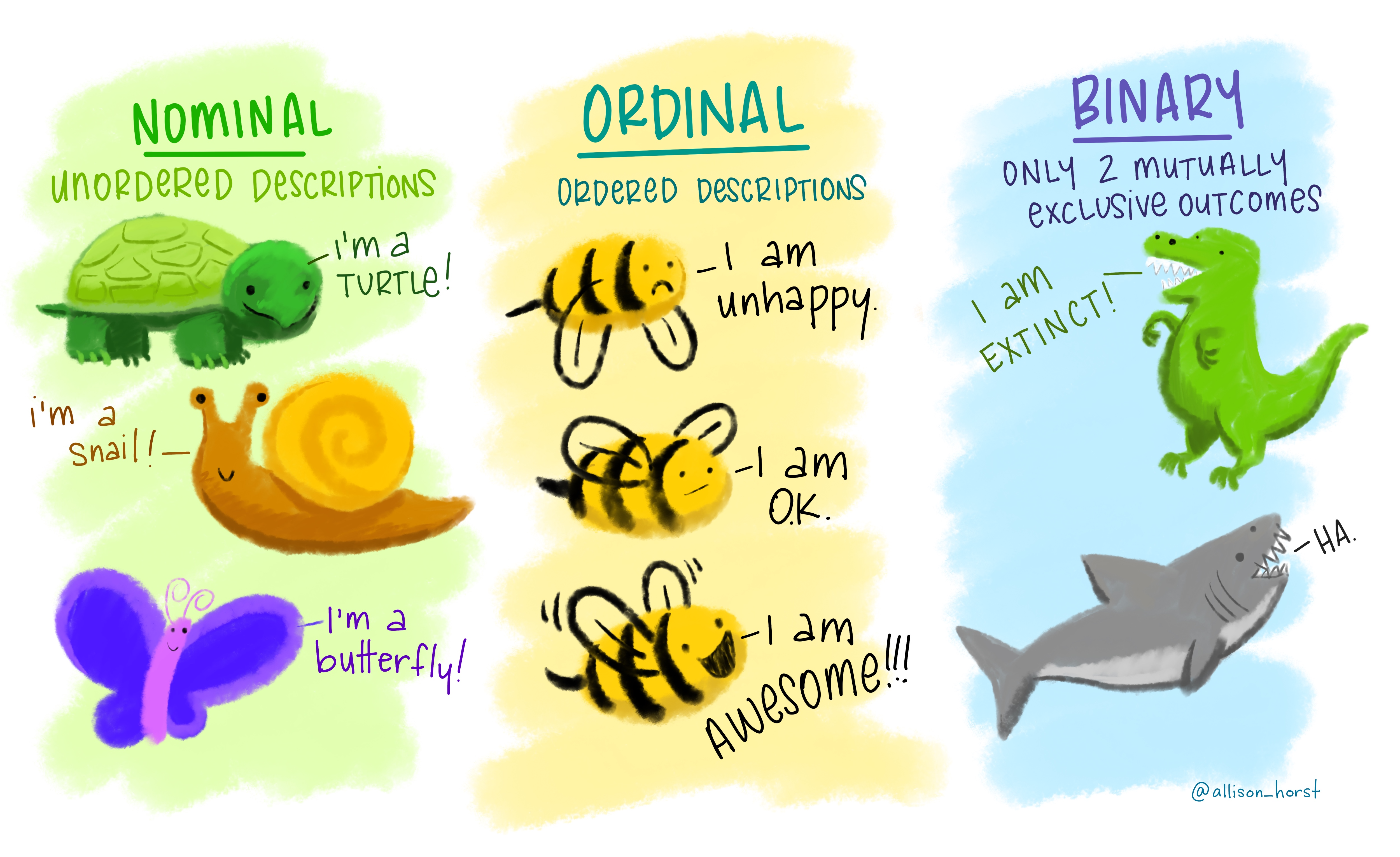
Factors are a special class of data specifically for categorical variables¹ which have a fixed, known, and mutually exclusive set of possible values².

Imagine we have a variable that records the month that an event occurred.

month <- c("Dec", "Apr", "Jan", "Mar")

The two main issues with coding this simply as a character string:

1. It doesn’t help catch spelling errors

month <- c("Dec", "Apr", "Jam", "Mar")

2. Characters are sorted alphabetically, which is not necessarily intuitive or useful for your variable

sort(month)

> [1] "Apr" "Dec" "Jan" "Mar"

1. For categoricals; forcats is also an anagram of factors.

2. Factors can also be created from character strings that you want to display in non-alphabetical order

Factors

Factors have an additional specification called levels. These are the categories of the categorical variable. We can create a vector of the levels first:

month_levels <- c(
  "Jan", "Feb", "Mar", "Apr", "May", "Jun", 
  "Jul", "Aug", "Sep", "Oct", "Nov", "Dec"
)

And then we can create a factor like so:

month_factor <- factor(month, levels = month_levels)
month_factor

> [1] Dec Apr Jan Mar
> Levels: Jan Feb Mar Apr May Jun Jul Aug Sep Oct Nov Dec

We can see that the levels specify in which order the categories should be displayed:

sort(month_factor)

> [1] Jan Mar Apr Dec
> Levels: Jan Feb Mar Apr May Jun Jul Aug Sep Oct Nov Dec

Creating Factors

factor is Base R’s function for creating factors while fct is forcats function for making factors. A couple of things to note about their differences:

factor

• Any values not specified as a level will be silently converted to NA
• Without specified levels, they’ll be created from the data in alphabetical order¹

fct

• Will send a error message if a value exists outside the specified levels
• Without specified levels, they’ll be created from the data in order of first appearance

You can create a factor by specifying col_factor() when reading in data with readr:

df <- read_csv(csv, col_types = cols(month = col_factor(month_levels)))

If you need to access the levels directly you can use the Base R function levels().

levels(month_factor)

>  [1] "Jan" "Feb" "Mar" "Apr" "May" "Jun" "Jul" "Aug" "Sep" "Oct" "Nov" "Dec"

1. This is risky to rely on since not every computer will sort strings the same way.

Changing the Order of Levels

One of the more common data manipulations you’ll want to do with factors is to change the ordering of the levels. This could be to put them in a more intuitive order but also to make a visualization clearer and more impactful.

Let’s use a subset of the General Social Survey¹ data to see what this might look like.

gss_cat

> # A tibble: 21,483 × 9
>     year marital         age race  rincome        partyid    relig denom tvhours
>    <int> <fct>         <int> <fct> <fct>          <fct>      <fct> <fct>   <int>
>  1  2000 Never married    26 White $8000 to 9999  Ind,near … Prot… Sout…      12
>  2  2000 Divorced         48 White $8000 to 9999  Not str r… Prot… Bapt…      NA
>  3  2000 Widowed          67 White Not applicable Independe… Prot… No d…       2
>  4  2000 Never married    39 White Not applicable Ind,near … Orth… Not …       4
>  5  2000 Divorced         25 White Not applicable Not str d… None  Not …       1
>  6  2000 Married          25 White $20000 - 24999 Strong de… Prot… Sout…      NA
>  7  2000 Never married    36 White $25000 or more Not str r… Chri… Not …       3
>  8  2000 Divorced         44 White $7000 to 7999  Ind,near … Prot… Luth…      NA
>  9  2000 Married          44 White $25000 or more Not str d… Prot… Other       0
> 10  2000 Married          47 White $25000 or more Strong re… Prot… Sout…       3
> # ℹ 21,473 more rows

1. Once you’ve loaded forcats you can run ?gss_cat to learn more.

Changing the Order of Levels

There are four related functions to change the level ordering in forcats.

fct_reorder()

1fct_reorder(.f = factor,
2            .x = ordering_vector,
3            .fun = optional_function)

1

factor is the factor to reorder (or a character string to be turned into a factor)

2

ordering_vector specifies how to reorder factor

3

optional_function is applied if there are multiple values of ordering_vector for each value of factor (the default is to take the median)

fct_relevel()

fct_relevel(.f = factor, 
4            ... = value,
5            after = placement)

4

value is either a function (i.e. sort) or a character level (default is to move it to the front of the vector)

5

placement is an optional vector index where the level should be placed

fct_reorder2()

fct_reorder2(.f = factor, 
6            .x = vector1,
            .y = vector2)

6

fct_reorder2 reorders factor by the values of vector2 associated with the largest values of vector1.

fct_infreq()

7fct_infreq(.f = factor)

7

fct_infreq reorders factor in decreasing frequency. See other variations here. Use with fct_rev() for increasing frequency.

Changing the Order of Levels

There are four related functions to change the level ordering in forcats.

• fct_reorder¹
• fct_relevel²
• fct_reorder2
• fct_infreq

fct_reorder() is for reordering levels by sorting along another variable

Without fct_reorder()

relig_summary <- gss_cat |>
  summarize(
    tvhours = mean(tvhours, na.rm = TRUE),
    .by = relig
  )

ggplot(relig_summary, aes(x = tvhours, y = relig)) + 
  geom_point()

With fct_reorder()

relig_summary |>
  mutate(
    relig = fct_reorder(relig, tvhours)
  ) |>
  ggplot(aes(x = tvhours, y = relig)) +
  geom_point()

fct_relevel() allows you to reorder the levels by hand

Without fct_relevel()

rincome_summary <- gss_cat |>
  summarize(
    age = mean(age, na.rm = TRUE),
    .by = rincome
  )

ggplot(rincome_summary, aes(x = age, y = rincome)) + 
  geom_point()

With fct_relevel()

ggplot(rincome_summary, aes(x = age, y = fct_relevel(rincome, "Not applicable"))) +
  geom_point()

fct_reorder2() is like fct_reorder(), except when the factor is mapped to a non-position aesthetic such as color

Without fct_reorder2()

by_age <- gss_cat |>
  filter(!is.na(age)) |> 
  count(age, marital) |>
  mutate(
    prop = n / sum(n), 
    .by = age
  )

ggplot(by_age, aes(x = age, y = prop, color = marital)) +
  geom_line(linewidth = 1) + 
  scale_color_brewer(palette = "Set1")

With fct_reorder()

ggplot(by_age, aes(x = age, y = prop, color = fct_reorder2(marital, age, prop))) +
  geom_line(linewidth = 1) +
  scale_color_brewer(palette = "Set1") + 
  labs(color = "marital") 

fct_infreq() reorders levels by the number of observations within each level (largest first)

Without fct_infreq()

gss_cat |>
  ggplot(aes(x = marital)) + 
  geom_bar()

With fct_infreq()

Question for you: what does fct_rev() do here?

gss_cat |>
  mutate(marital = marital |> fct_infreq() |> fct_rev()) |>
  ggplot(aes(x = marital)) +
  geom_bar()

1. Use fct_reorder and fct_reorder2 for categorical variables where ordering is arbitary.

2. Use fct_relevel for categorical variables that already have an inherent ordering.

Changing the Value of Levels

You may also want to change the actual values of your factor levels. The main way to do this is fct_recode().

8gss_cat |> count(partyid)

8

You can use count() to get the full list of levels for a variable and their respective counts.

> # A tibble: 10 × 2
>    partyid                n
>    <fct>              <int>
>  1 No answer            154
>  2 Don't know             1
>  3 Other party          393
>  4 Strong republican   2314
>  5 Not str republican  3032
>  6 Ind,near rep        1791
>  7 Independent         4119
>  8 Ind,near dem        2499
>  9 Not str democrat    3690
> 10 Strong democrat     3490

fct_recode()

gss_cat |>
  mutate(
    partyid = fct_recode(partyid,
      "Republican, strong" = "Strong republican",
      "Republican, weak" = "Not str republican",
      "Independent, near rep" = "Ind,near rep",
      "Independent, near dem" = "Ind,near dem",
      "Democrat, weak" = "Not str democrat",
      "Democrat, strong" = "Strong democrat"
    )
  ) |>
  count(partyid)

> # A tibble: 10 × 2
>    partyid                   n
>    <fct>                 <int>
>  1 No answer               154
>  2 Don't know                1
>  3 Other party             393
>  4 Republican, strong     2314
>  5 Republican, weak       3032
>  6 Independent, near rep  1791
>  7 Independent            4119
>  8 Independent, near dem  2499
>  9 Democrat, weak         3690
> 10 Democrat, strong       3490

Some features of fct_recode():

• Will leave the levels that aren’t explicitly mentioned, as is.
• Will warn you if you accidentally refer to a level that doesn’t exist.
• You can combine groups by assigning multiple old levels to the same new level.

fct_collapse()

A useful variant of fct_recode() is fct_collapse() which will allow you to collapse a lot of levels at once.

gss_cat |>
  mutate(
    partyid = fct_collapse(partyid,
      "other" = c("No answer", "Don't know", "Other party"),
      "rep" = c("Strong republican", "Not str republican"),
      "ind" = c("Ind,near rep", "Independent", "Ind,near dem"),
      "dem" = c("Not str democrat", "Strong democrat")
    )
  ) |>
  count(partyid)

> # A tibble: 4 × 2
>   partyid     n
>   <fct>   <int>
> 1 other     548
> 2 rep      5346
> 3 ind      8409
> 4 dem      7180

fct_lump_*

Sometimes you’ll have several levels of a variable that have a small enough N to warrant grouping them together into an other category. The family of fct_lump_* functions are designed to help with this.

gss_cat |>
9  mutate(relig = fct_lump_n(relig, n = 10)) |>
  count(relig, sort = TRUE)

9

Other functions include: fct_lump_min(), fct_lump_prop(), fct_lump_lowfreq(). Read more about them here.

> # A tibble: 10 × 2
>    relig                       n
>    <fct>                   <int>
>  1 Protestant              10846
>  2 Catholic                 5124
>  3 None                     3523
>  4 Christian                 689
>  5 Other                     458
>  6 Jewish                    388
>  7 Buddhism                  147
>  8 Inter-nondenominational   109
>  9 Moslem/islam              104
> 10 Orthodox-christian         95

Ordered Factors

So far we’ve mostly been discussing how to code nominal variables, or categorical variables that have no inherent ordering.

If you want to specify that your factor has a strict order you can classify it as a ordered factor.

10ordered(c("a", "b", "c"))

10

Ordered factors imply a strict ordering and equal distance between levels: the first level is “less than” the second level by the same amount that the second level is “less than” the third level, and so on.

> [1] a b c
> Levels: a < b < c

In practice there are only two ways in which ordered factors are different than factors:

1. scale_color_viridis()/scale_fill_viridis() will be used automatically when mapping an ordered factored in ggplot2 because it implies an ordered ranking
2. If you use an ordered function in a linear model, it will use “polygonal contrasts”. You can learn more about what this means here.

Numbers

Numbers, Two Ways

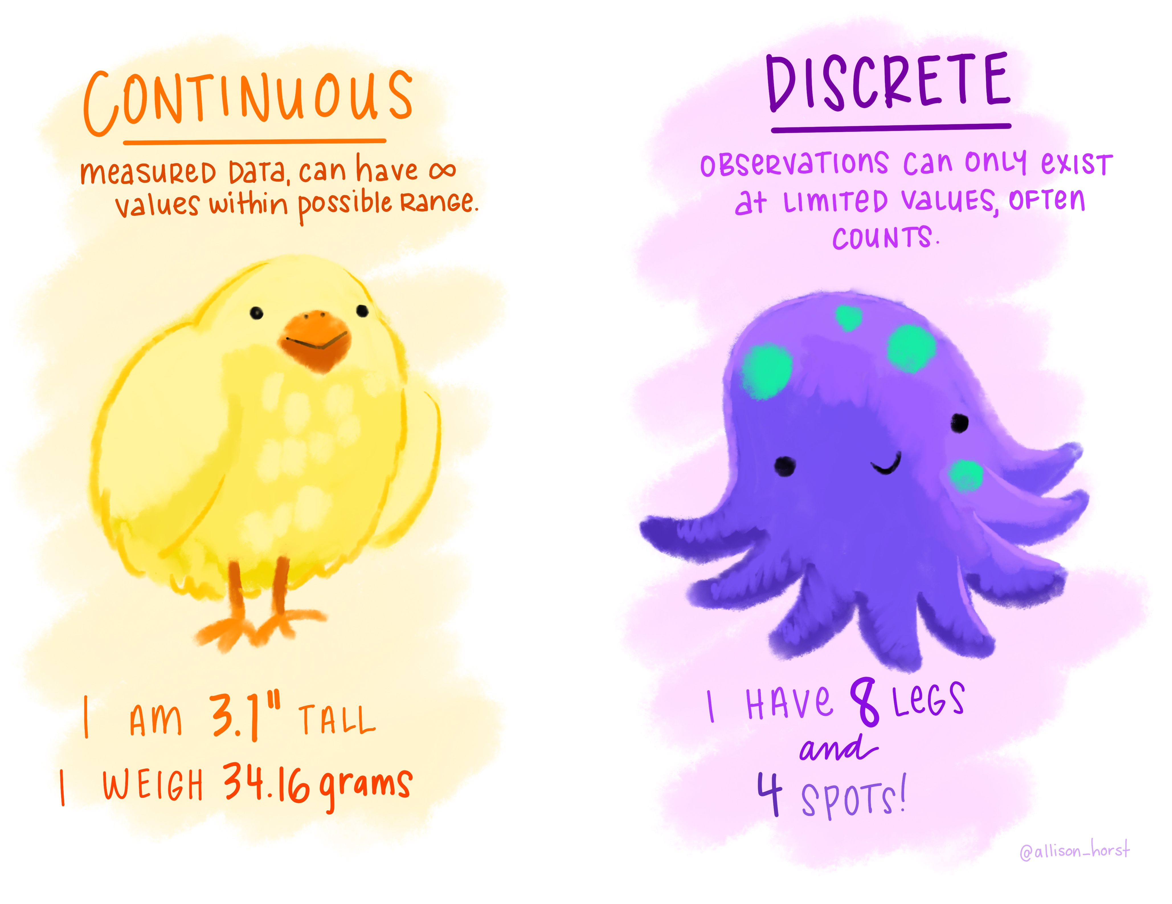
R has two types of numeric variables: double and integer.

• Integers must be round numbers while doubles can be decimals
• They are stored differently, and arithmetic works a bit differently with integers vs doubles
• Continuous values must be stored as doubles
• Discrete values can be integers, doubles, or factors

Numbers Coded as Character Strings

Oftentimes numerical data is coded as a string so you’ll need to use the appropriate parsing function to read it in in the correct form.

parse_integer(c("1", "2", "3"))

> [1] 1 2 3

parse_double(c("1", "2", "3.123"))

> [1] 1.000 2.000 3.123

If you have values with extraneous non-numerical text you want to ignore there’s a separate function for that.

parse_number(c("USD 3,513", "59%", "$1,123,456.00"))

> [1]    3513      59 1123456

count()

A very useful and common exploratory data analysis tool is to check the relative sums of different categories of a variable. That’s what count() is for!

library(nycflights13)
data(flights)

1flights |> count(origin)

1

Add the argument sort = TRUE to see the most common values first (i.e. arranged in descending order). . . .

> # A tibble: 3 × 2
>   origin      n
>   <chr>   <int>
> 1 EWR    120835
> 2 JFK    111279
> 3 LGA    104662

This is functionally the same as grouping and summarizing with n().

flights |> 
2  summarise(n= n(),
3            .by = origin)

2

n() is a special summary function that doesn’t take any arguments and instead accesses information about the “current” group. This means that it only works inside dplyr verbs.

3

You can do this longer version if you also want to compute other summaries simultaneously.

> # A tibble: 3 × 2
>   origin      n
>   <chr>   <int>
> 1 EWR    120835
> 2 LGA    104662
> 3 JFK    111279

n_distinct()

Use this function if you want the count the number of distinct (unique) values of one or more variables.

Say we’re interested in which destinations are served by the most carriers:

flights |> 
  summarize(carriers = n_distinct(carrier), 
            .by = dest) |> 
  arrange(desc(carriers))

> # A tibble: 105 × 2
>    dest  carriers
>    <chr>    <int>
>  1 ATL          7
>  2 ORD          7
>  3 TPA          7
>  4 BOS          7
>  5 CLT          7
>  6 IAD          6
>  7 MSP          6
>  8 DTW          6
>  9 MSY          6
> 10 PIT          6
> # ℹ 95 more rows

Weighted Counts

A weighted count is simply a grouped sum, therefore count has a wt argument to allow for the shorthand.

How many miles did each plane fly?

flights |> 
  summarize(miles = sum(distance), 
            .by = tailnum)

> # A tibble: 4,044 × 2
>    tailnum  miles
>    <chr>    <dbl>
>  1 N14228  171713
>  2 N24211  172934
>  3 N619AA   32141
>  4 N804JB  311992
>  5 N668DN   50352
>  6 N39463  169905
>  7 N516JB  359585
>  8 N829AS   52549
>  9 N593JB  377619
> 10 N3ALAA   67925
> # ℹ 4,034 more rows

This is equivalent to:

flights |> count(tailnum, wt = distance) 

> # A tibble: 4,044 × 2
>    tailnum      n
>    <chr>    <dbl>
>  1 D942DN    3418
>  2 N0EGMQ  250866
>  3 N10156  115966
>  4 N102UW   25722
>  5 N103US   24619
>  6 N104UW   25157
>  7 N10575  150194
>  8 N105UW   23618
>  9 N107US   21677
> 10 N108UW   32070
> # ℹ 4,034 more rows

Other Useful Arithmetic Functions

In addition to the standards (+, -, /, *, ^), R has many other useful arithmetic functions.

Pairwise min/max

mydata <- tribble(
  ~x, ~y,
  1,  3,
  5,  2,
  7, NA,
)
mydata

> # A tibble: 3 × 2
>       x     y
>   <dbl> <dbl>
> 1     1     3
> 2     5     2
> 3     7    NA

mydata |> 
  mutate(
    min = min(x, y, na.rm = TRUE),
    max = max(x, y, na.rm = TRUE)
  )

> # A tibble: 3 × 4
>       x     y   min   max
>   <dbl> <dbl> <dbl> <dbl>
> 1     1     3     1     7
> 2     5     2     1     7
> 3     7    NA     1     7

mydata |> 
  mutate(
6    min = pmin(x, y, na.rm = TRUE),
7    max = pmax(x, y, na.rm = TRUE)
  )

6

pmin() returns the smallest value in each row. min(), by contrast, finds the smallest observation given a number of rows.

7

pmax() returns the largest value in each row. max(), by contrast, finds the largest observation given a number of rows.

> # A tibble: 3 × 4
>       x     y   min   max
>   <dbl> <dbl> <dbl> <dbl>
> 1     1     3     1     3
> 2     5     2     2     5
> 3     7    NA     7     7

Other Useful Arithmetic Functions

Modular arithmetic

81:10 %/% 3

8

Computes integer division.

>  [1] 0 0 1 1 1 2 2 2 3 3

91:10 %% 3

9

Computes the remainder.

>  [1] 1 2 0 1 2 0 1 2 0 1

We can see how this can be useful in our flights data which has curiously stored time:

flights |> mutate(hour = sched_dep_time %/% 100,
                  minute = sched_dep_time %% 100,
                  .keep = "used")

> # A tibble: 336,776 × 3
>    sched_dep_time  hour minute
>             <int> <dbl>  <dbl>
>  1            515     5     15
>  2            529     5     29
>  3            540     5     40
>  4            545     5     45
>  5            600     6      0
>  6            558     5     58
>  7            600     6      0
>  8            600     6      0
>  9            600     6      0
> 10            600     6      0
> # ℹ 336,766 more rows

Other Useful Arithmetic Functions

Logarithms¹

10log(c(2.718282, 7.389056, 20.085537))

10

Inverse is exp()

> [1] 1 2 3

11log2(c(2, 4, 8))

11

Easy to interpret because a difference of 1 on the log scale corresponds to doubling on the original scale and a difference of -1 corresponds to halving. Inverse is 2^.

> [1] 1 2 3

12log10(c(10, 100, 1000))

12

Easy to back-transform because everything is on the order of 10. Inverse is 10^.

> [1] 1 2 3

1. An incredibly useful transformation for dealing with data that ranges across multiple orders of magnitude and converting exponential growth to linear growth.

Other Useful Arithmetic Functions

Cumulative and Rolling Aggregates

Base R provides cumsum(), cumprod(), cummin(), cummax() for running, or cumulative, sums, products, mins and maxes. dplyr provides cummean() for cumulative means.

1:15

>  [1]  1  2  3  4  5  6  7  8  9 10 11 12 13 14 15

13cumsum(1:15)

13

cumsum() is the most common in practice.

>  [1]   1   3   6  10  15  21  28  36  45  55  66  78  91 105 120

For complex rolling/sliding aggregates, check out the slidr package.

Other Useful Arithmetic Functions

Numeric Ranges

x <- c(1, 2, 5, 10, 15, 20)
14cut(x, breaks = c(0, 5, 10, 15, 20))

14

cut() breaks up (aka bins) a numeric vector into discrete buckets

> [1] (0,5]   (0,5]   (0,5]   (5,10]  (10,15] (15,20]
> Levels: (0,5] (5,10] (10,15] (15,20]

15cut(x, breaks = c(0, 5, 10, 100))

15

The bins don’t have to be the same size.

> [1] (0,5]    (0,5]    (0,5]    (5,10]   (10,100] (10,100]
> Levels: (0,5] (5,10] (10,100]

cut(x, 
  breaks = c(0, 5, 10, 15, 20), 
16  labels = c("sm", "md", "lg", "xl")
)

16

You can optionally supply your own labels. Note that there should be one less labels than breaks.

> [1] sm sm sm md lg xl
> Levels: sm md lg xl

17y <- c(NA, -10, 5, 10, 30)
cut(y, breaks = c(0, 5, 10, 15, 20))

17

Any values outside of the range of the breaks will become NA.

> [1] <NA>   <NA>   (0,5]  (5,10] <NA>  
> Levels: (0,5] (5,10] (10,15] (15,20]

Rounding

round() allows us to round to a certain decimal place. Without specifying an argument for the digits argument it will round to the nearest integer.

round(pi)

> [1] 3

round(pi, digits = 2)

> [1] 3.14

Using negative integers in the digits argument allows you to round on the left-hand side of the decimal place.

round(39472, digits = -1)

> [1] 39470

round(39472, digits = -2)

> [1] 39500

round(39472, digits = -3)

> [1] 39000

Rounding

What’s going on here?

round(c(1.5, 2.5)) 

> [1] 2 2

round() uses what’s known as “round half to even” or Banker’s rounding: if a number is half way between two integers, it will be rounded to the even integer. This is a good strategy because it keeps the rounding unbiased: half of all 0.5s are rounded up, and half are rounded down.

floor() and ceiling() are also useful rounding shortcuts.

18floor(123.456)

18

Always rounds down.

> [1] 123

19ceiling(123.456)

19

Always rounds up.

> [1] 124

Summary Functions

Central Tendency

20x <- sample(1:500, size = 100, replace = TRUE)
mean(x)

20

sample() takes a vector of data, and samples size elements from it, with replacement if replace equals TRUE.

> [1] 253.48

median(x)

> [1] 269

21quantile(x, .95)

21

A generalization of the median: quantile(x, 0.95) will find the value that’s greater than 95% of the values; quantile(x, 0.5) is equivalent to the median.

> 95% 
> 490

Summary Functions

Measures of Spread/Variation

min(x)

> [1] 1

max(x)

> [1] 500

range(x)

> [1]   1 500

22IQR(x)

22

Equivalent to quantile(x, 0.75) - quantile(x, 0.25) and gives you the range that contains the middle 50% of the data.

> [1] 263.5

23var(x)

23

\[s^2 = \frac{\sum(x_i-\overline{x})^2}{n-1}\]

> [1] 23404.15

24sd(x)

24

\[s = \sqrt{\frac{\sum(x_i-\overline{x})^2}{n-1}}\]

> [1] 152.9842

Common Numerical Manipulations

These formulas can be used in a summary call but are also useful with mutate(), particularly if being applied to grouped data.

19x / sum(x)
20(x - mean(x)) / sd(x)
21(x - min(x)) / (max(x) - min(x))
22x / first(x)

19

Calculates the proportion of a total.

20

Computes a Z-score (standardized to mean 0 and sd 1).

21

Standardizes to range [0, 1].

22

Computes an index based on the first observation.

Summary Functions

Positions

first(x)

> [1] 319

last(x)

> [1] 3

nth(x, n = 77)

> [1] 6

These are all really helpful but is there a good summary descriptive statistics function?

Basic summary statistics

summary(iris)

>   Sepal.Length    Sepal.Width     Petal.Length    Petal.Width   
>  Min.   :4.300   Min.   :2.000   Min.   :1.000   Min.   :0.100  
>  1st Qu.:5.100   1st Qu.:2.800   1st Qu.:1.600   1st Qu.:0.300  
>  Median :5.800   Median :3.000   Median :4.350   Median :1.300  
>  Mean   :5.843   Mean   :3.057   Mean   :3.758   Mean   :1.199  
>  3rd Qu.:6.400   3rd Qu.:3.300   3rd Qu.:5.100   3rd Qu.:1.800  
>  Max.   :7.900   Max.   :4.400   Max.   :6.900   Max.   :2.500  
>        Species  
>  setosa    :50  
>  versicolor:50  
>  virginica :50  
>                 
>                 
> 

Better summary statistics

A basic example:

library(skimr)
skim(iris)

Data summary

Name	iris
Number of rows	150
Number of columns	5
_______________________
Column type frequency:
factor	1
numeric	4
________________________
Group variables	None

Variable type: factor

skim_variable	n_missing	complete_rate	ordered	n_unique	top_counts
Species	0	1	FALSE	3	set: 50, ver: 50, vir: 50

Variable type: numeric

skim_variable	n_missing	complete_rate	mean	sd	p0	p25	p50	p75	p100	hist
Sepal.Length	0	1	5.84	0.83	4.3	5.1	5.80	6.4	7.9	▆▇▇▅▂
Sepal.Width	0	1	3.06	0.44	2.0	2.8	3.00	3.3	4.4	▁▆▇▂▁
Petal.Length	0	1	3.76	1.77	1.0	1.6	4.35	5.1	6.9	▇▁▆▇▂
Petal.Width	0	1	1.20	0.76	0.1	0.3	1.30	1.8	2.5	▇▁▇▅▃

Better summary statistics

A more complex example:

skim(starwars)

Data summary

Name	starwars
Number of rows	87
Number of columns	14
_______________________
Column type frequency:
character	8
list	3
numeric	3
________________________
Group variables	None

Variable type: character

skim_variable	n_missing	complete_rate	min	max	empty	n_unique	whitespace
name	0	1.00	3	21	0	87	0
hair_color	5	0.94	4	13	0	11	0
skin_color	0	1.00	3	19	0	31	0
eye_color	0	1.00	3	13	0	15	0
sex	4	0.95	4	14	0	4	0
gender	4	0.95	8	9	0	2	0
homeworld	10	0.89	4	14	0	48	0
species	4	0.95	3	14	0	37	0

Variable type: list

skim_variable	n_missing	complete_rate	n_unique	min_length	max_length
films	0	1	24	1	7
vehicles	0	1	11	0	2
starships	0	1	16	0	5

Variable type: numeric

skim_variable	n_missing	complete_rate	mean	sd	p0	p25	p50	p75	p100	hist
height	6	0.93	174.60	34.77	66	167.0	180	191.0	264	▂▁▇▅▁
mass	28	0.68	97.31	169.46	15	55.6	79	84.5	1358	▇▁▁▁▁
birth_year	44	0.49	87.57	154.69	8	35.0	52	72.0	896	▇▁▁▁▁

skim function

Highlights of this summary statistics function:

• provides a larger set of statistics than summary() including number missing, complete, n, sd, histogram for numeric data
• presentation is in a compact, organized format
• reports each data type separately
• handles a wide range of data classes including dates, logicals, strings, lists and more
• can be used with summary() for an overall summary of the data (w/o specifics about columns)
• individual columns can be selected for a summary of only a subset of the data
• handles grouped data
• behaves nicely in pipelines
• produces knitted results for documents
• easily and highly customizable (i.e. specify your own statistics and classes)

Missing Values

Explicit Missing Values

An explicit missing value is the presence of an absence.

In other words, an explicit missing value is one in which you see an NA.

Depending on the reason for its missingness, there are different ways to deal with NAs.

Data Entry Shorthand

If your data were entered by hand and NAs merely represent a value being carried forward from the last entry then you can use fill() to help complete your data.

treatment <- tribble(
  ~person,           ~treatment, ~response,
  "Derrick Whitmore", 1,         7,
  NA,                 2,         10,
  "Katherine Burke",  3,         NA,
  NA,                 1,         4
)

treatment |>
1  fill(everything())

1

fill() takes one or more variables (in this case everything(), which means all variables), and by default fills them in downwards. If you have a different issue you can change the .direction argument to "up","downup", or "updown".

> # A tibble: 4 × 3
>   person           treatment response
>   <chr>                <dbl>    <dbl>
> 1 Derrick Whitmore         1        7
> 2 Derrick Whitmore         2       10
> 3 Katherine Burke          3       10
> 4 Katherine Burke          1        4

Explicit Missing Values

Represent A Fixed Value

Other times an NA represents some fixed value, usually 0.

x <- c(1, 4, 5, 7, NA)
2coalesce(x, 0)

2

coalesce() in the dplyr package takes a vector as the first argument and will replace any missing values with the value provided in the second argument.

> [1] 1 4 5 7 0

Represented By a Fixed Value

If the opposite issue occurs (i.e. a value is actually an NA), try specifying that to the na argument of your readr data import function. Otherwise, use na_if() from dplyr.

x <- c(1, 4, 5, 7, -99)
na_if(x, -99)

> [1]  1  4  5  7 NA

Explicit Missing Values

NaNs

A special sub-type of missing value is an NaN, or Not a Number.

These generally behave similar to NAs and are likely the result of a mathematical operation that has an indeterminate result:

0 / 0 

> [1] NaN

0 * Inf

> [1] NaN

Inf - Inf

> [1] NaN

sqrt(-1)

> [1] NaN

If you need to explicitly identify an NaN you can use is.nan().

Implicit NAs

An implicit missing value is the absence of a presence.

We’ve seen a couple of ways that implicit NAs can be made explicit in previous lectures: pivoting and joining.

For example, if we really look at the dataset below, we can see that there are missing values that don’t appear as NA merely due to the current structure of the data.

stocks

> # A tibble: 7 × 3
>    year   qtr price
>   <dbl> <dbl> <dbl>
> 1  2020     1  1.88
> 2  2020     2  0.59
> 3  2020     3  0.35
> 4  2020     4  0.89
> 5  2021     2  0.34
> 6  2021     3  0.17
> 7  2021     4  2.66

Implicit NAs

tidyr::complete() allows you to generate explicit missing values by providing a set of variables that define the combination of rows that should exist.

stocks |>
  complete(year, qtr)

> # A tibble: 8 × 3
>    year   qtr price
>   <dbl> <dbl> <dbl>
> 1  2020     1  1.88
> 2  2020     2  0.59
> 3  2020     3  0.35
> 4  2020     4  0.89
> 5  2021     1 NA   
> 6  2021     2  0.34
> 7  2021     3  0.17
> 8  2021     4  2.66

stocks |>
  complete(year, qtr, fill = list(price = 0.93))

> # A tibble: 8 × 3
>    year   qtr price
>   <dbl> <dbl> <dbl>
> 1  2020     1  1.88
> 2  2020     2  0.59
> 3  2020     3  0.35
> 4  2020     4  0.89
> 5  2021     1  0.93
> 6  2021     2  0.34
> 7  2021     3  0.17
> 8  2021     4  2.66

The fill argument of complete only allows you to supply 1 value per variable. If you have more than one value to fill, use complete to create the data structure you need, and case_when to replace NAs would be the most straightforward approach.

Missing Factor Levels

The last type of missingness is a theoretical level of a factor that doesn’t have any observations.

For instance, we have this health dataset and we’re interested in smokers:

health

> # A tibble: 5 × 3
>   name    smoker   age
>   <chr>   <fct>  <dbl>
> 1 Ikaia   no        34
> 2 Oletta  no        88
> 3 Leriah  no        75
> 4 Dashay  no        47
> 5 Tresaun no        56

health |> count(smoker)

> # A tibble: 1 × 2
>   smoker     n
>   <fct>  <int>
> 1 no         5

3levels(health$smoker)

3

This dataset only contains non-smokers, but we know that smokers exist; the group of smokers is simply empty.

> [1] "yes" "no"

4health |> count(smoker, .drop = FALSE)

4

We can request count() to keep all the groups, even those not seen in the data by using .drop = FALSE.

> # A tibble: 2 × 2
>   smoker     n
>   <fct>  <int>
> 1 yes        0
> 2 no         5

Missing Factors in Plots

This sample principle applies when visualizing a factor variable, which will automatically drop levels that don’t have any values. Use drop_values = FALSE in the appropriate scale to display implicit NAs.

ggplot(health, aes(x = smoker)) +
  geom_bar() +
  scale_x_discrete() + 
  theme_classic(base_size = 22)

ggplot(health, aes(x = smoker)) +
  geom_bar() +
  scale_x_discrete(drop = FALSE) + 
  theme_classic(base_size = 22)

Testing Data Types

There are also functions to test for certain data types:

is.numeric(5)

> [1] TRUE

is.character("A")

> [1] TRUE

is.logical(TRUE)

> [1] TRUE

is.infinite(-Inf)

> [1] TRUE

is.na(NA)

> [1] TRUE

is.nan(NaN)

> [1] TRUE

Going deeper into the abyss (aka NAs)

Artwork by @allison_horst

Going deeper into the abyss (aka NAs)

A lot has been written about NAs and if they are a feature of your data you’re likely going to have to spend a great deal of time thinking about how they arose¹ and if/how they bias your data.

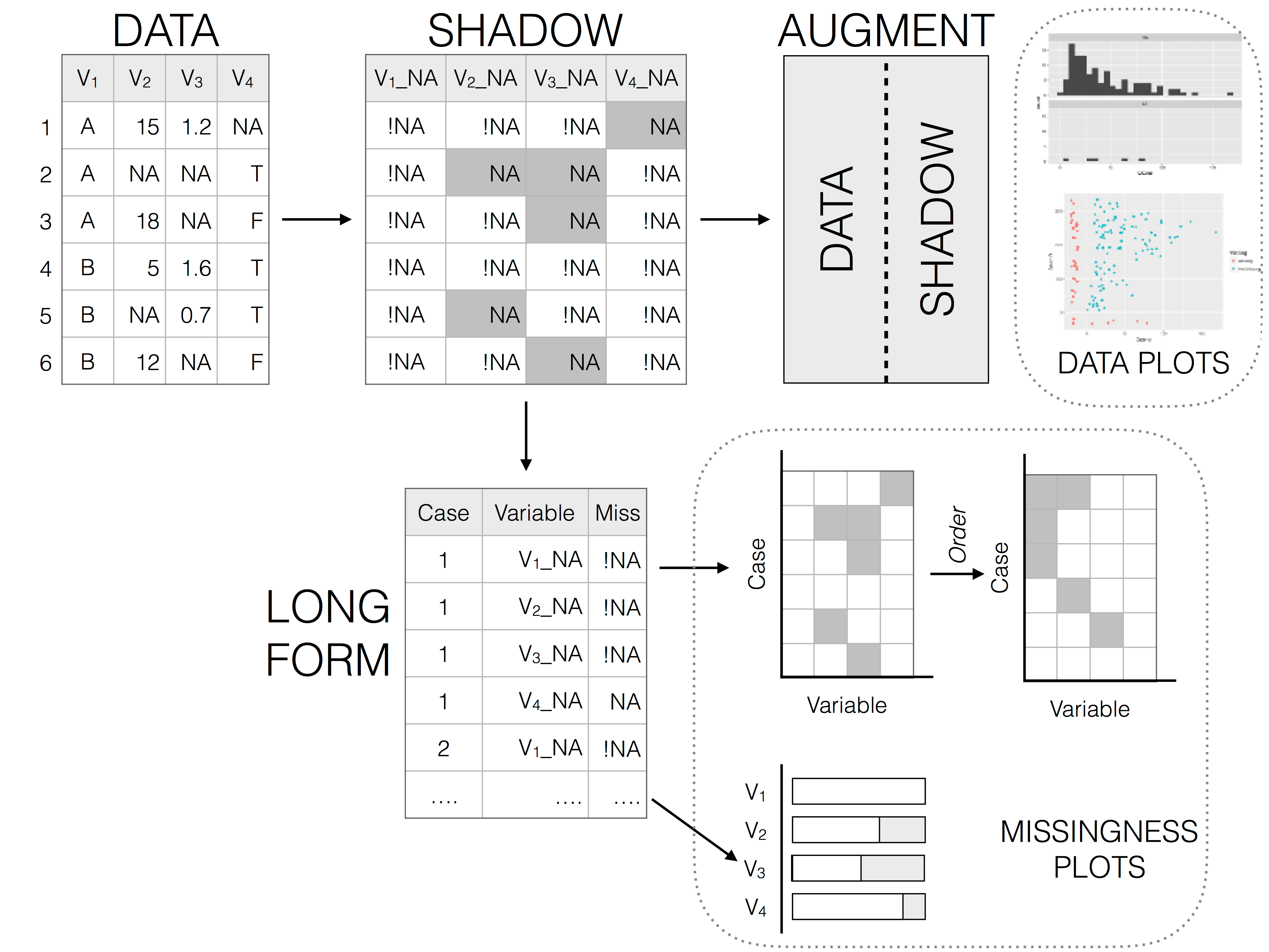
The best package for really exploring your NAs is naniar, which provides tidyverse-style syntax for summarizing, visualizing, and manipulating missing data.

It provides the following for missing data:

• a special data structure
• shorthand and numerical summaries (in variables and cases)
• visualizations

1. Missing Completely at Random? Missing at Random? Missing Not at Random? Read more about the differences here.

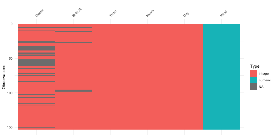
naniar examples

See more here.

visdat example

library(visdat)
vis_dat(airquality)

You can read more about this package and its functionality here. For an tidy-style approach for imputing missing values check out the simputation package.

Break!

Vectors

Making Vectors

In R, we call a set of values of the same type a vector. We can create vectors using the c() function (“c” for combine or concatenate).

c(1, 3, 7, -0.5)

> [1]  1.0  3.0  7.0 -0.5

Vectors have one dimension: length

length(c(1, 3, 7, -0.5))

> [1] 4

All elements of a vector are the same type (e.g. numeric or character)!

Character data is the lowest denomination so anything mixed with it will be converted to a character.

Generating Numeric Vectors

There are shortcuts for generating numeric vectors:

1:10

>  [1]  1  2  3  4  5  6  7  8  9 10

1seq(-3, 6, by = 1.75)

1

Sequence from -3 to 6, increments of 1.75

> [1] -3.00 -1.25  0.50  2.25  4.00  5.75

2rep(c(0, 1), times = 3)
3rep(c(0, 1), each = 3)
4rep(c(0, 1), length.out = 3)

2

Repeat c(0, 1) 3 times.

3

Repeat each element 3 times.

4

Repeat c(0, 1) until the length of the final vector is 3.

> [1] 0 1 0 1 0 1
> [1] 0 0 0 1 1 1
> [1] 0 1 0

You can also assign values to a vector using Base R indexing rules.

x <- c(3, 6, 2, 9, 5)
x[6] <- 8
x

> [1] 3 6 2 9 5 8

x[c(7, 8)] <- c(9, 9)
x

> [1] 3 6 2 9 5 8 9 9

Element-wise Vector Math

When doing arithmetic operations on vectors, R handles these element-wise:

c(1, 2, 3) + c(4, 5, 6)

> [1] 5 7 9

5c(1, 2, 3, 4)^3

5

Exponentiation is carried out using the ^ operator.

> [1]  1  8 27 64

Other common operations: *, /, exp() = \(e^x\), log() = \(\log_e(x)\)

Recycling Rules

R handles mismatched lengths of vectors by recycling, or repeating, the short vector.

x <- c(1, 2, 10, 20)
6x / 5

6

This is shorthand for: x / c(5, 5, 5, 5)

> [1] 0.2 0.4 2.0 4.0

You generally only want to recycle scalars, or vectors of length 1. Technically, however, R will recycle any vector that’s shorter in length (and it won’t always give you a warning that that’s what it’s doing, i.e. if the longer vector is not a multiple of the shorter vector).

x * c(1, 2)

> [1]  1  4 10 40

x * c(1, 2, 3)

> Warning in x * c(1, 2, 3): longer object length is not a multiple of shorter
> object length

> [1]  1  4 30 20

Recycling with Logicals

The same rules apply to logical operations which can lead to unexpected results without warning.

For example, take this code which attempts to find all flights in January and February:

flights |> 
  mutate(rowID = 1:nrow(flights)) |> 
  relocate(rowID) |>
7  filter(month == c(1, 2))

7

A common mistake is to mix up == with %in%. This code will actually find flights in odd numbered rows that departed in January and flights in even numbered rows that departed in February. Unfortunately there’s no warning because flights has an even number of rows.

> # A tibble: 25,977 × 20
>    rowID  year month   day dep_time sched_dep_time dep_delay arr_time
>    <int> <int> <int> <int>    <int>          <int>     <dbl>    <int>
>  1     1  2013     1     1      517            515         2      830
>  2     3  2013     1     1      542            540         2      923
>  3     5  2013     1     1      554            600        -6      812
>  4     7  2013     1     1      555            600        -5      913
>  5     9  2013     1     1      557            600        -3      838
>  6    11  2013     1     1      558            600        -2      849
>  7    13  2013     1     1      558            600        -2      924
>  8    15  2013     1     1      559            600        -1      941
>  9    17  2013     1     1      559            600        -1      854
> 10    19  2013     1     1      600            600         0      837
> # ℹ 25,967 more rows
> # ℹ 12 more variables: sched_arr_time <int>, arr_delay <dbl>, carrier <chr>,
> #   flight <int>, tailnum <chr>, origin <chr>, dest <chr>, air_time <dbl>,
> #   distance <dbl>, hour <dbl>, minute <dbl>, time_hour <dttm>

To protect you from this type of silent failure, most tidyverse functions use a stricter form of recycling that only recycles single values. However, when using base R functions like ==, this protection is not built in.

Example: Standardizing Data

Let’s say we had some test scores and we wanted to put these on a standardized scale:

\[z_i = \frac{x_i - \text{mean}(x)}{\text{SD}(x)}\]

x <- c(97, 68, 75, 77, 69, 81)
z <- (x - mean(x)) / sd(x)
round(z, 2)

> [1]  1.81 -0.93 -0.27 -0.08 -0.83  0.30

Math with Missing Values

Even one NA “poisons the well”: You’ll get NA out of your calculations unless you add the extra argument na.rm = TRUE (available in some functions):

vector_w_missing <- c(1, 2, NA, 4, 5, 6, NA)
mean(vector_w_missing)

> [1] NA

mean(vector_w_missing, na.rm = TRUE)

> [1] 3.6

Subsetting Vectors

Recall, we can subset a vector in a number of ways:

• Passing a single index or vector of entries to keep:

first_names <- c("Andre", "Brady", "Cecilia", "Danni", "Edgar", "Francie")
first_names[c(1, 2)]

> [1] "Andre" "Brady"

• Passing a single index or vector of entries to drop:

first_names[-3]

> [1] "Andre"   "Brady"   "Danni"   "Edgar"   "Francie"

• Passing a logical condition:

8first_names[nchar(first_names) == 7]

8

nchar() counts the number of characters in a character string.

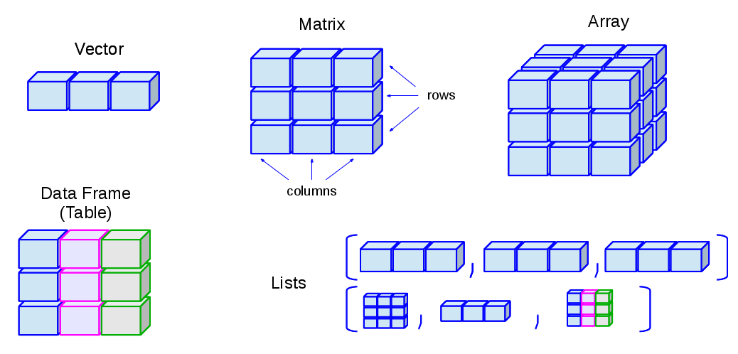
> [1] "Cecilia" "Francie"

• Passing a named vector:

pet_names <- c(dog = "Lemon", cat = "Seamus")
pet_names["cat"]

>      cat 
> "Seamus"

Matrices

Matrices: Two Dimensions

Matrices extend vectors to two dimensions: rows and columns. We can construct them directly using matrix().

R fills in a matrix column-by-column (not row-by-row!)

a_matrix <- matrix(first_names, nrow = 2, ncol = 3)
a_matrix

>      [,1]    [,2]      [,3]     
> [1,] "Andre" "Cecilia" "Edgar"  
> [2,] "Brady" "Danni"   "Francie"

Similar to vectors, you can make assignments using Base R indexing methods.

a_matrix[1, c(1:3)] <- c("Hakim", "Tony", "Eduardo")
a_matrix

>      [,1]    [,2]    [,3]     
> [1,] "Hakim" "Tony"  "Eduardo"
> [2,] "Brady" "Danni" "Francie"

However, you can’t add rows or columns to a matrix in this way. You can only reassign already-existing cell values.

a_matrix[3, c(1:3)] <- c("Lucille", "Hanif", "June")

> Error in `[<-`(`*tmp*`, 3, c(1:3), value = c("Lucille", "Hanif", "June": subscript out of bounds

Binding Vectors

We can also make matrices by binding vectors together with rbind() (row bind) and cbind() (column bind).

b_matrix <- rbind(c(1, 2, 3), c(4, 5, 6))
b_matrix

>      [,1] [,2] [,3]
> [1,]    1    2    3
> [2,]    4    5    6

c_matrix <- cbind(c(1, 2), c(3, 4), c(5, 6))
c_matrix

>      [,1] [,2] [,3]
> [1,]    1    3    5
> [2,]    2    4    6

Subsetting Matrices

We subset matrices using the same methods as with vectors, except we index them with [rows, columns]¹:

a_matrix

>      [,1]    [,2]    [,3]     
> [1,] "Hakim" "Tony"  "Eduardo"
> [2,] "Brady" "Danni" "Francie"

9a_matrix[1, 2]

9

Row 1, Column 2.

> [1] "Tony"

10a_matrix[1, c(2,3)]

10

Row 1, Columns 2 and 3.

> [1] "Tony"    "Eduardo"

We can obtain the dimensions of a matrix using dim().

dim(a_matrix)

> [1] 2 3

1. Like we learned how to do with dataframes in week 3.

Matrices Becoming Vectors

If a matrix ends up having just one row or column after subsetting, by default R will make it into a vector.

a_matrix[, 1] 

> [1] "Hakim" "Brady"

You can prevent this behavior using drop = FALSE.

a_matrix[, 1, drop = FALSE] 

>      [,1]   
> [1,] "Hakim"
> [2,] "Brady"

Matrix Data Type Warning

Matrices can contain numeric, integer, factor, character, or logical. But just like vectors, all elements must be the same data type.

bad_matrix <- cbind(1:2, c("apple", "banana"))
bad_matrix

>      [,1] [,2]    
> [1,] "1"  "apple" 
> [2,] "2"  "banana"

In this case, everything was converted to characters!

Matrix Dimension Names

We can access dimension names or name them ourselves:

rownames(bad_matrix) <- c("First", "Last")
colnames(bad_matrix) <- c("Number", "Name")
bad_matrix

>       Number Name    
> First "1"    "apple" 
> Last  "2"    "banana"

11bad_matrix[ ,"Name", drop = FALSE]

11

drop = FALSE maintains the matrix structure; when drop = TRUE (the default) it will be converted to a vector.

>       Name    
> First "apple" 
> Last  "banana"

Matrix Arithmetic

Matrices of the same dimensions can have math performed element-wise with the usual arithmetic operators:

matrix(c(2, 4, 6, 8),nrow = 2, ncol = 2) / matrix(c(2, 1, 3, 1),nrow = 2, ncol = 2)

>      [,1] [,2]
> [1,]    1    2
> [2,]    4    8

“Proper” Matrix Math

To do matrix transpositions, use t().

c_matrix

>      [,1] [,2] [,3]
> [1,]    1    3    5
> [2,]    2    4    6

e_matrix <- t(c_matrix)
e_matrix

>      [,1] [,2]
> [1,]    1    2
> [2,]    3    4
> [3,]    5    6

To do actual matrix multiplication¹ (not element-wise), use %*%.

f_matrix <- c_matrix %*% e_matrix 
f_matrix

>      [,1] [,2]
> [1,]   35   44
> [2,]   44   56

1. A reminder of how to do matrix multiplication :)

“Proper” Matrix Math

To invert an invertible square matrix¹, use solve().

g_matrix <- solve(f_matrix)
g_matrix

>           [,1]      [,2]
> [1,]  2.333333 -1.833333
> [2,] -1.833333  1.458333

1. A reminder of how to invert a 2x2 square matrix.

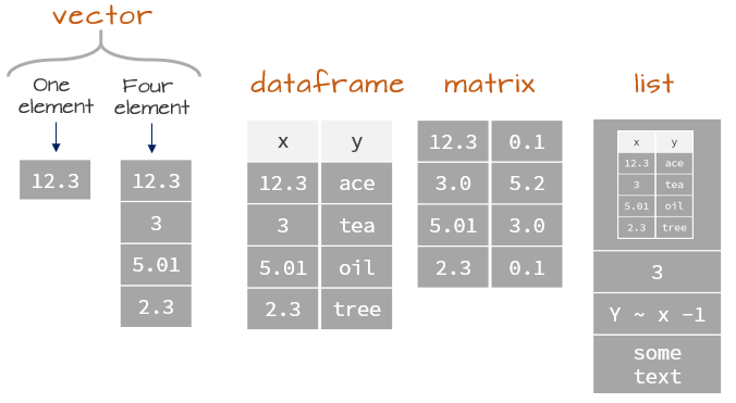
Matrices vs. Data.frames and Tibbles

All of these structures display data in two dimensions

• matrix

  • Base R
  • Single data type allowed

• data.frame

  • Base R
  • Stores multiple data types
  • Default for data storage

• tibbles

  • tidyverse
  • Stores multiple data types
  • Displays nicely

In practice, data.frames and tibbles are very similar!

Creating data.frames or tibbles

We can create a data.frame or tibble by specifying the columns separately, as individual vectors:

data.frame(Column1 = c(1, 2, 3),
           Column2 = c("A", "B", "C"))

>   Column1 Column2
> 1       1       A
> 2       2       B
> 3       3       C

tibble(Column1 = c(1, 2, 3),
       Column2 = c("A", "B", "C"))

> # A tibble: 3 × 2
>   Column1 Column2
>     <dbl> <chr>  
> 1       1 A      
> 2       2 B      
> 3       3 C

Note: data.frames and tibbles allow for mixed data types!

This distinction leads us to the final data type, of which data.frames and tibbles are a particular subset.

tibble’s additional advantages are only displaying the first 10 rows and only the columns that will comfortably fit within the parameters of your console space when called (data.frame will display all columns and a certain number of rows depending upon your default max setting - usually this is an overwhelming amount of output, aesthetically confusing, and not very helpful).

Lists

What are Lists?

Lists are objects that can store multiple types of data.

my_list <- list(first_thing = 1:5,
                second_thing = matrix(8:11, nrow = 2), 
                third_thing = fct(c("apple", "pear", "banana", "apple", "apple")))
my_list

> $first_thing
> [1] 1 2 3 4 5
> 
> $second_thing
>      [,1] [,2]
> [1,]    8   10
> [2,]    9   11
> 
> $third_thing
> [1] apple  pear   banana apple  apple 
> Levels: apple pear banana

Accessing List Elements

You can access a list element by its name or number in [[ ]], or a $ followed by its name:

my_list[["first_thing"]]

> [1] 1 2 3 4 5

my_list[[1]]

> [1] 1 2 3 4 5

my_list$first_thing

> [1] 1 2 3 4 5

Why Two Brackets [[ ]]?

Double brackets get the actual element — as whatever data type it is stored as, in that location in the list.

str(my_list[[1]])

>  int [1:5] 1 2 3 4 5

If you use single brackets to access list elements, you get a list back.

str(my_list[1])

> List of 1
>  $ first_thing: int [1:5] 1 2 3 4 5

names() and List Elements

You can use names() to get a vector of list element names:

names(my_list)

> [1] "first_thing"  "second_thing" "third_thing"

pluck()

An alternative to using Base R’s [[ ]] is using pluck() from the tidyverse’s purrr package.

obj1 <- list("a", list(1, elt = "foo"))
obj2 <- list("b", list(2, elt = "bar"))
x <- list(obj1, obj2)
x

> [[1]]
> [[1]][[1]]
> [1] "a"
> 
> [[1]][[2]]
> [[1]][[2]][[1]]
> [1] 1
> 
> [[1]][[2]]$elt
> [1] "foo"
> 
> 
> 
> [[2]]
> [[2]][[1]]
> [1] "b"
> 
> [[2]][[2]]
> [[2]][[2]][[1]]
> [1] 2
> 
> [[2]][[2]]$elt
> [1] "bar"

pluck(x, 1) 

> [[1]]
> [1] "a"
> 
> [[2]]
> [[2]][[1]]
> [1] 1
> 
> [[2]]$elt
> [1] "foo"

This is the same as same as x[[1]].

pluck()

An alternative to using Base R’s [[ ]] is using pluck() from the tidyverse’s purrr package.

obj1 <- list("a", list(1, elt = "foo"))
obj2 <- list("b", list(2, elt = "bar"))
x <- list(obj1, obj2)
x

> [[1]]
> [[1]][[1]]
> [1] "a"
> 
> [[1]][[2]]
> [[1]][[2]][[1]]
> [1] 1
> 
> [[1]][[2]]$elt
> [1] "foo"
> 
> 
> 
> [[2]]
> [[2]][[1]]
> [1] "b"
> 
> [[2]][[2]]
> [[2]][[2]][[1]]
> [1] 2
> 
> [[2]][[2]]$elt
> [1] "bar"

pluck(x, 1, 2) 

> [[1]]
> [1] 1
> 
> $elt
> [1] "foo"

This is the same as x[[1]][[2]].

pluck()

An alternative to using Base R’s [[ ]] is using pluck() from the tidyverse’s purrr package.

obj1 <- list("a", list(1, elt = "foo"))
obj2 <- list("b", list(2, elt = "bar"))
x <- list(obj1, obj2)
x

> [[1]]
> [[1]][[1]]
> [1] "a"
> 
> [[1]][[2]]
> [[1]][[2]][[1]]
> [1] 1
> 
> [[1]][[2]]$elt
> [1] "foo"
> 
> 
> 
> [[2]]
> [[2]][[1]]
> [1] "b"
> 
> [[2]][[2]]
> [[2]][[2]][[1]]
> [1] 2
> 
> [[2]][[2]]$elt
> [1] "bar"

pluck(x, 1, 2, "elt") 

> [1] "foo"

You can supply names as indices if the vectors are named. This is the same as calling x[[1]][[2]][["elt"]].

Example: Regression Output

When you perform linear regression in R, the output is a list!

lm_output <- lm(speed ~ dist, data = cars)
is.list(lm_output)

> [1] TRUE

names(lm_output)

>  [1] "coefficients"  "residuals"     "effects"       "rank"         
>  [5] "fitted.values" "assign"        "qr"            "df.residual"  
>  [9] "xlevels"       "call"          "terms"         "model"

lm_output$coefficients

> (Intercept)        dist 
>   8.2839056   0.1655676

What does a list object look like?

str(lm_output)

> List of 12
>  $ coefficients : Named num [1:2] 8.284 0.166
>   ..- attr(*, "names")= chr [1:2] "(Intercept)" "dist"
>  $ residuals    : Named num [1:50] -4.62 -5.94 -1.95 -4.93 -2.93 ...
>   ..- attr(*, "names")= chr [1:50] "1" "2" "3" "4" ...
>  $ effects      : Named num [1:50] -108.894 29.866 -0.501 -3.945 -1.797 ...
>   ..- attr(*, "names")= chr [1:50] "(Intercept)" "dist" "" "" ...
>  $ rank         : int 2
>  $ fitted.values: Named num [1:50] 8.62 9.94 8.95 11.93 10.93 ...
>   ..- attr(*, "names")= chr [1:50] "1" "2" "3" "4" ...
>  $ assign       : int [1:2] 0 1
>  $ qr           :List of 5
>   ..$ qr   : num [1:50, 1:2] -7.071 0.141 0.141 0.141 0.141 ...
>   .. ..- attr(*, "dimnames")=List of 2
>   .. .. ..$ : chr [1:50] "1" "2" "3" "4" ...
>   .. .. ..$ : chr [1:2] "(Intercept)" "dist"
>   .. ..- attr(*, "assign")= int [1:2] 0 1
>   ..$ qraux: num [1:2] 1.14 1.15
>   ..$ pivot: int [1:2] 1 2
>   ..$ tol  : num 1e-07
>   ..$ rank : int 2
>   ..- attr(*, "class")= chr "qr"
>  $ df.residual  : int 48
>  $ xlevels      : Named list()
>  $ call         : language lm(formula = speed ~ dist, data = cars)
>  $ terms        :Classes 'terms', 'formula'  language speed ~ dist
>   .. ..- attr(*, "variables")= language list(speed, dist)
>   .. ..- attr(*, "factors")= int [1:2, 1] 0 1
>   .. .. ..- attr(*, "dimnames")=List of 2
>   .. .. .. ..$ : chr [1:2] "speed" "dist"
>   .. .. .. ..$ : chr "dist"
>   .. ..- attr(*, "term.labels")= chr "dist"
>   .. ..- attr(*, "order")= int 1
>   .. ..- attr(*, "intercept")= int 1
>   .. ..- attr(*, "response")= int 1
>   .. ..- attr(*, ".Environment")=<environment: R_GlobalEnv> 
>   .. ..- attr(*, "predvars")= language list(speed, dist)
>   .. ..- attr(*, "dataClasses")= Named chr [1:2] "numeric" "numeric"
>   .. .. ..- attr(*, "names")= chr [1:2] "speed" "dist"
>  $ model        :'data.frame':    50 obs. of  2 variables:
>   ..$ speed: num [1:50] 4 4 7 7 8 9 10 10 10 11 ...
>   ..$ dist : num [1:50] 2 10 4 22 16 10 18 26 34 17 ...
>   ..- attr(*, "terms")=Classes 'terms', 'formula'  language speed ~ dist
>   .. .. ..- attr(*, "variables")= language list(speed, dist)
>   .. .. ..- attr(*, "factors")= int [1:2, 1] 0 1
>   .. .. .. ..- attr(*, "dimnames")=List of 2
>   .. .. .. .. ..$ : chr [1:2] "speed" "dist"
>   .. .. .. .. ..$ : chr "dist"
>   .. .. ..- attr(*, "term.labels")= chr "dist"
>   .. .. ..- attr(*, "order")= int 1
>   .. .. ..- attr(*, "intercept")= int 1
>   .. .. ..- attr(*, "response")= int 1
>   .. .. ..- attr(*, ".Environment")=<environment: R_GlobalEnv> 
>   .. .. ..- attr(*, "predvars")= language list(speed, dist)
>   .. .. ..- attr(*, "dataClasses")= Named chr [1:2] "numeric" "numeric"
>   .. .. .. ..- attr(*, "names")= chr [1:2] "speed" "dist"
>  - attr(*, "class")= chr "lm"

Data Structures in R Overview

Data Structures in R Overview

Lab

Matrices and Lists

1. Write code to create the following matrix:

>      [,1] [,2] [,3]
> [1,] "A"  "B"  "C" 
> [2,] "D"  "E"  "F"

2. Write a line of code to extract the second column. Ensure the output is still a matrix.

>      [,1]
> [1,] "B" 
> [2,] "E"

3. Complete the following sentence: “Lists are to vectors, what data frames are to…”

4. Create a list that contains 3 elements:

   1. ten_numbers (integers between 1 and 10)
   2. my_name (your name as a character)
   3. booleans (vector of TRUE and FALSE alternating three times)

Answers

1. Write code to create the following matrix:

matrix_test <- matrix(c("A", "B", "C", "D", "E", "F"), nrow = 2, byrow = TRUE)
matrix_test

>      [,1] [,2] [,3]
> [1,] "A"  "B"  "C" 
> [2,] "D"  "E"  "F"

2. Write a line of code to extract the second column. Ensure the output is still a matrix.

matrix_test[ ,2, drop = FALSE]

>      [,1]
> [1,] "B" 
> [2,] "E"

Answers

3. Complete the following sentence: “Lists are to vectors, what data frames are to…Matrices!¹”

4. Create a list that contains 3 elements: So many ways to do this! Here’s one example.

things_I_like <- list(
  numbers = 8,
  animals = c("birds", "frogs", "lizards"),
  foods = rep("pasta", 10))
things_I_like

> $numbers
> [1] 8
> 
> $animals
> [1] "birds"   "frogs"   "lizards"
> 
> $foods
>  [1] "pasta" "pasta" "pasta" "pasta" "pasta" "pasta" "pasta" "pasta" "pasta"
> [10] "pasta"

1. Lists and data frames can contain mixed data types, while vectors and matrices can only contain one data type. Additionally, lists and vectors are technically one dimension while matrices and dataframes are two dimensions.

Homework