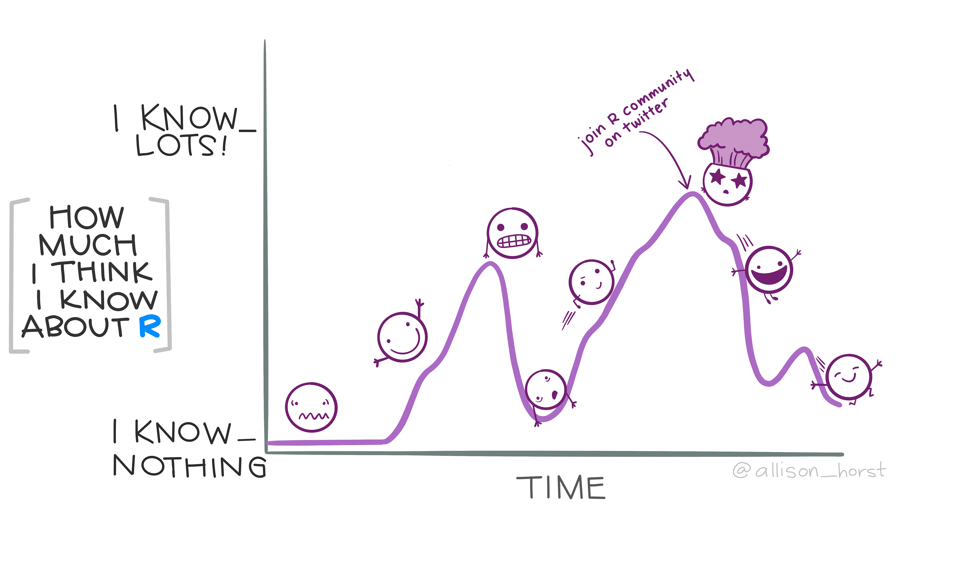
You’ve already learned SO MUCH in this class:
But if grad school teaches us anything, it’s that the more we learn, the more we realize how much more there is to learn. 🥴😑🫠
This can be freeing! And even fun?! Let your curiosity run wild!
Modeling in R

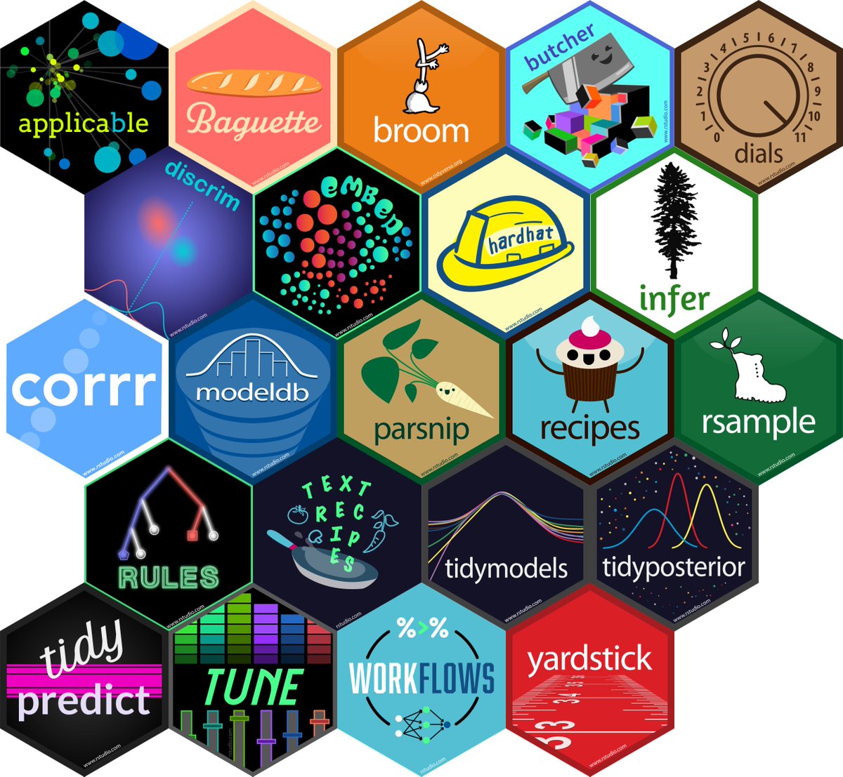
tidymodels packages
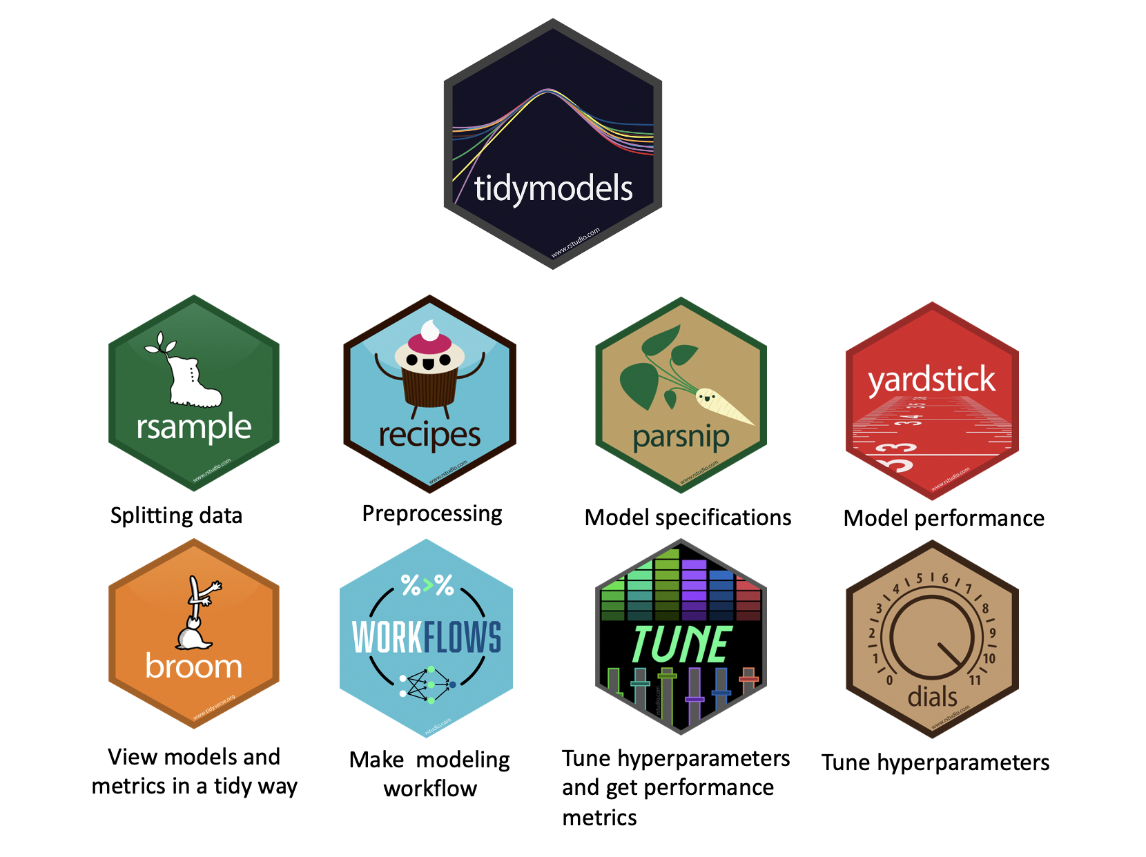
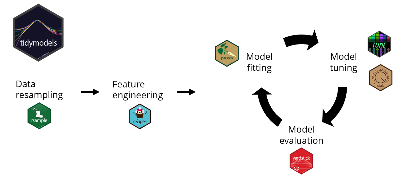
tidymodels approach
Packages using tidymodels framework
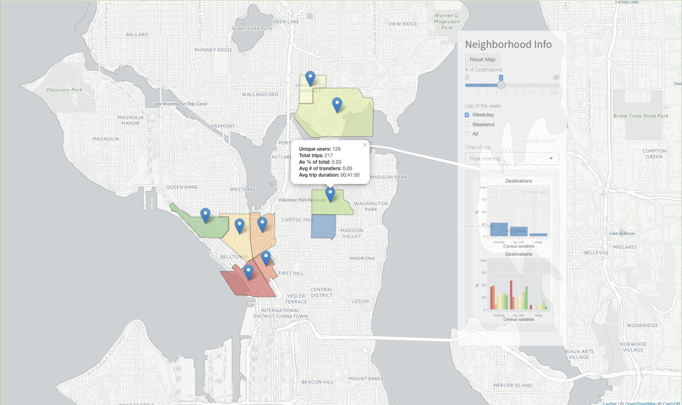
Making a map
Once we have data we want to visualize we can call ggmap to visualize the spatial area and layer on any geoms/stats as you would with ggplot2.
bbox <- make_bbox(lon, lat,
4                  data = violent_crimes)
map <- get_stadiamap( bbox = bbox,
                      maptype = "stamen_toner_lite",
5                      zoom = 14 )

ggmap(map) +
  geom_point(data = violent_crimes,
6 color = "red")- 4
- Creating the bounding box for the longitude and latitude.
- 5
- Retrieving the map with specifications.
- 6
-
The only difference with layers using
ggmapis that (1) you need to specify the data arguments in the layers and (2) the spatial aestheticsxandyare set tolonandlat, respectively. (If they’re named something different in your dataset, just putmapping = aes(x = longitude, y = latitude), for example.)

Using different geoms

Marginal histogram
library(ggExtra)
data(mpg, package = "ggplot2")

mpg_select <- mpg |>
  filter(hwy >= 35 & cty > 27)
g <- ggplot(mpg, aes(cty, hwy)) +
  geom_count() +
  geom_smooth(method = "lm", se = F) +
  theme_bw()
7ggMarginal(g, type = "histogram", fill = "transparent")- 7
- Code that adds marginal plot.

Marginal boxplot
library(ggExtra)
data(mpg, package = "ggplot2")

mpg_select <- mpg |>
  filter(hwy >= 35 & cty > 27)
g <- ggplot(mpg, aes(cty, hwy)) +
  geom_count() +
  geom_smooth(method = "lm", se = F) +
  theme_bw()
7ggMarginal(g, type = "boxplot", fill = "transparent")- 7
- Code that adds marginal plot.

Marginal density curve
library(ggExtra)
data(mpg, package = "ggplot2")

mpg_select <- mpg |>
  filter(hwy >= 35 & cty > 27)
g <- ggplot(mpg, aes(cty, hwy)) +
  geom_count() +
  geom_smooth(method = "lm", se = F) +
  theme_bw()
7ggMarginal(g, type = "density", fill = "transparent")- 7
- Code that adds marginal plot.

Create animations
Shiny
Shiny is an open source R package that provides an elegant and powerful web framework for building web applications using R. Shiny helps you turn your analyses into interactive web applications without requiring HTML, CSS, or JavaScript knowledge.
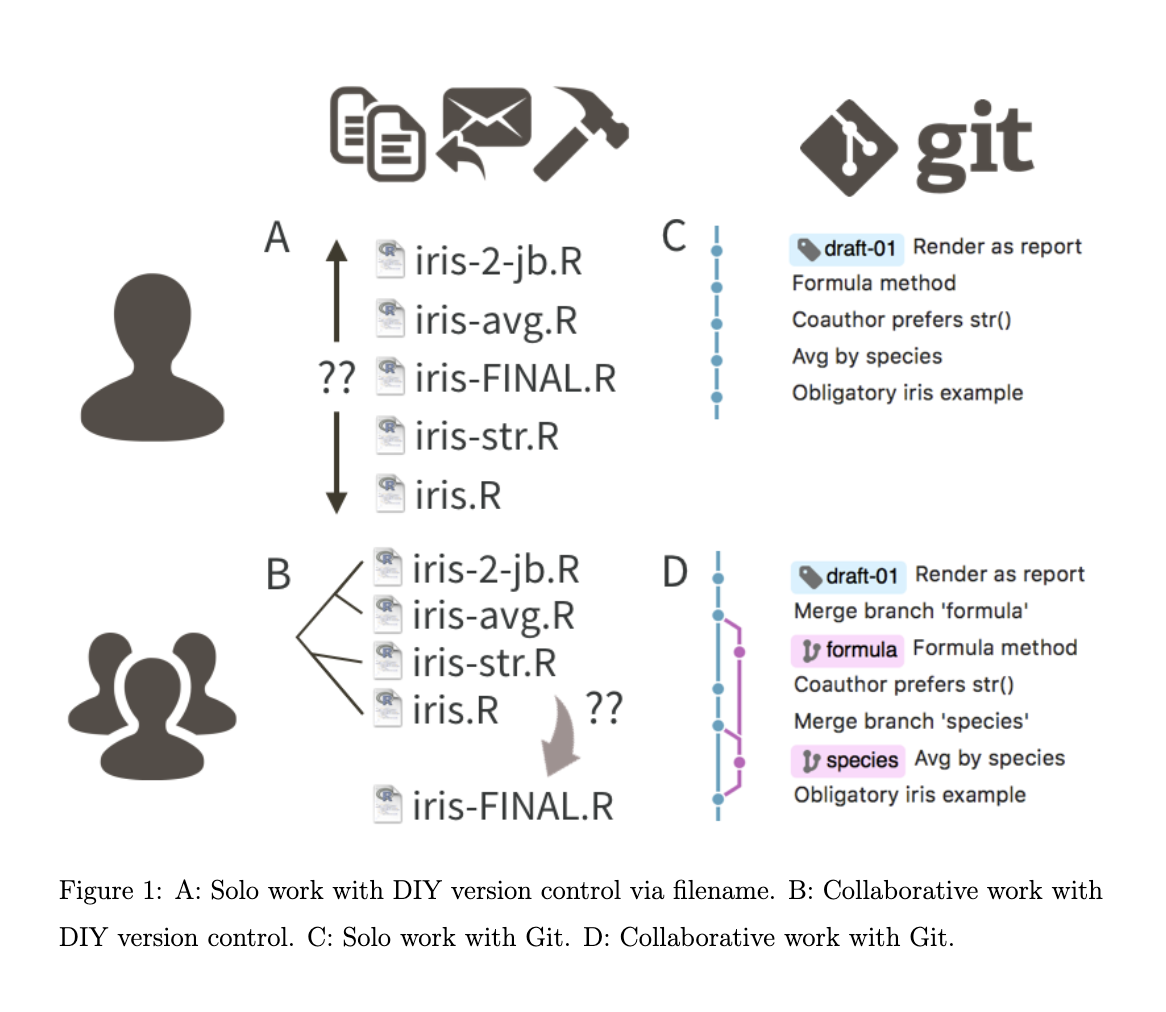
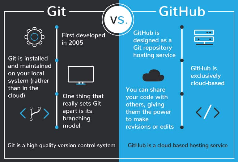
What is version control?
Version control allows you to work work individually and/or collaboratively in a highly structured, documented way.
It’s basically like a robust save program for your project. You track and log changes you make over time and the version control system allows you to review or even restore earlier versions of your project.
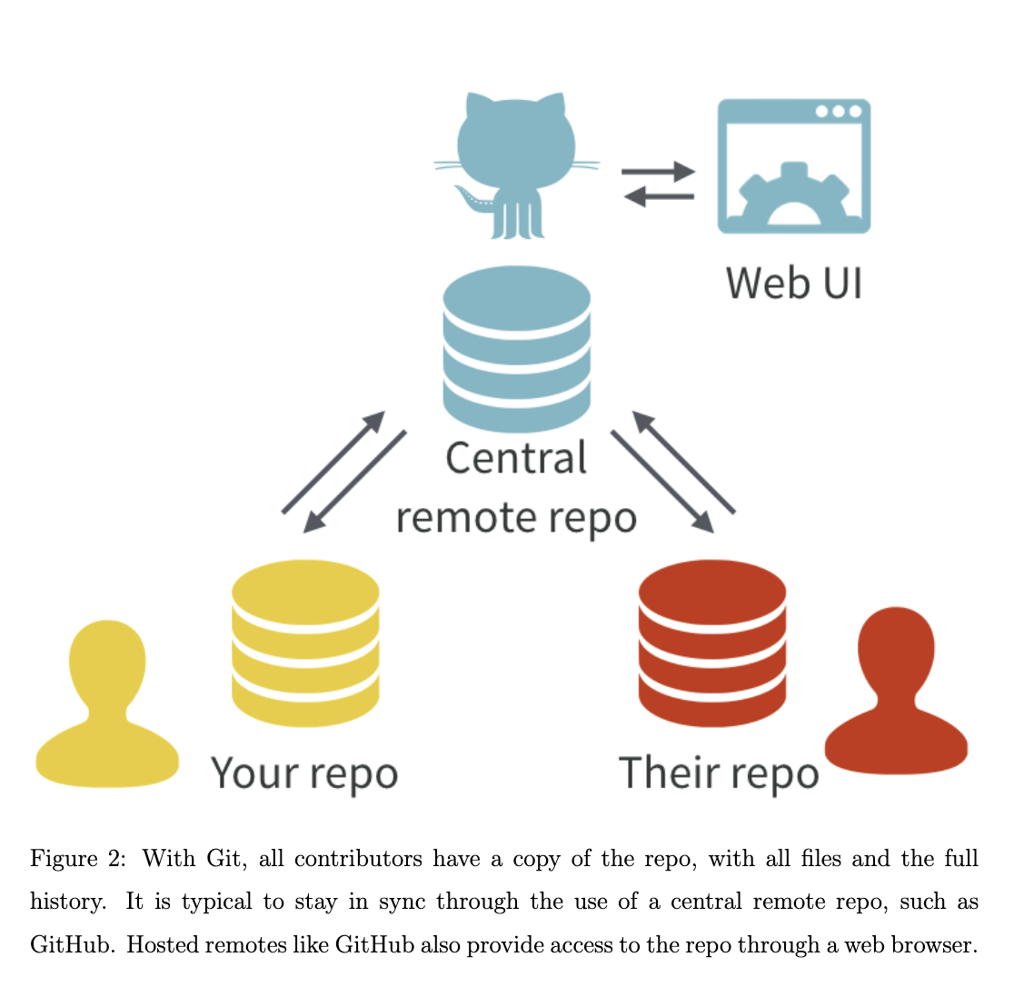
Originally meant for software developers, git has been adopted by computational social scientists to source code but also to keep track of the whole collection of files that make up a research project.

Why use version control?
What is Github?
Why use Github?

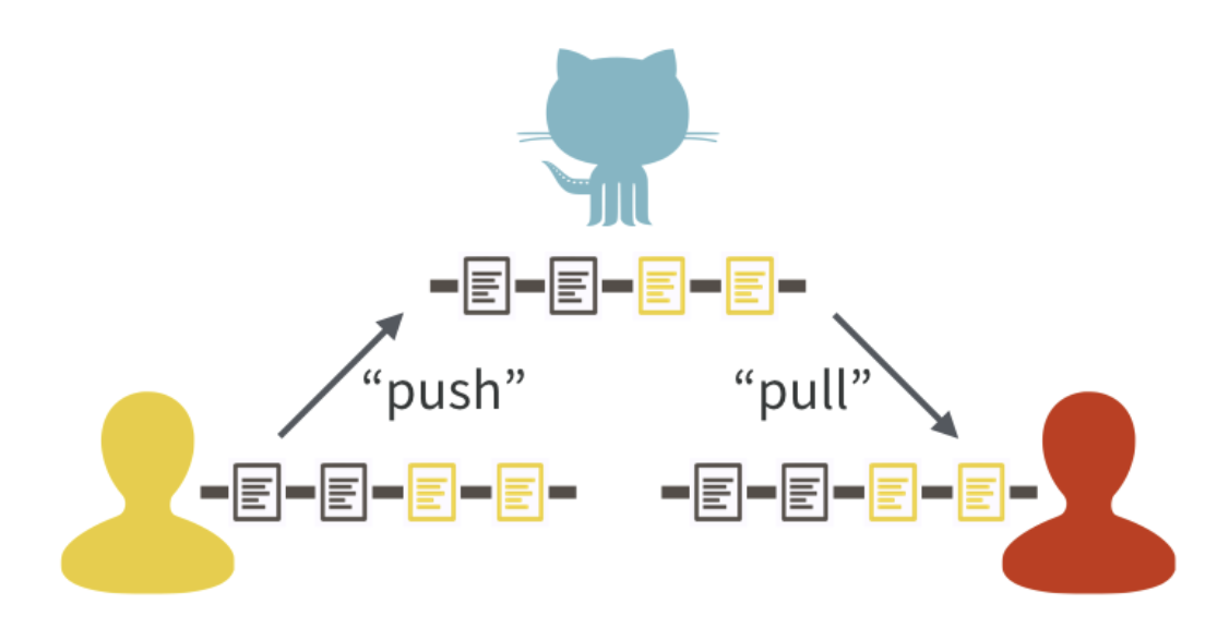
Collaboration made “easier”
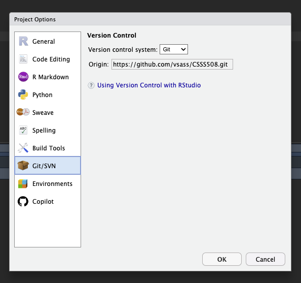
Git integration with R Studio
Thanks for spending so much time this quarter learning with me 😎
Don’t forget to fill out the course evaluation that you received via email!