Let’s start by getting to know each other a bit better. Share the following with your neighbor:
Name and pronouns
Program and year
Experience with programming (in R or more generally)
One word that best describes your feelings about taking this class
If you could have any superpower, what would you choose?
Pair up with someone nearby and introduce yourself to one another (~ 5 min).
Some reasons I love R, RStudio, and Quarto
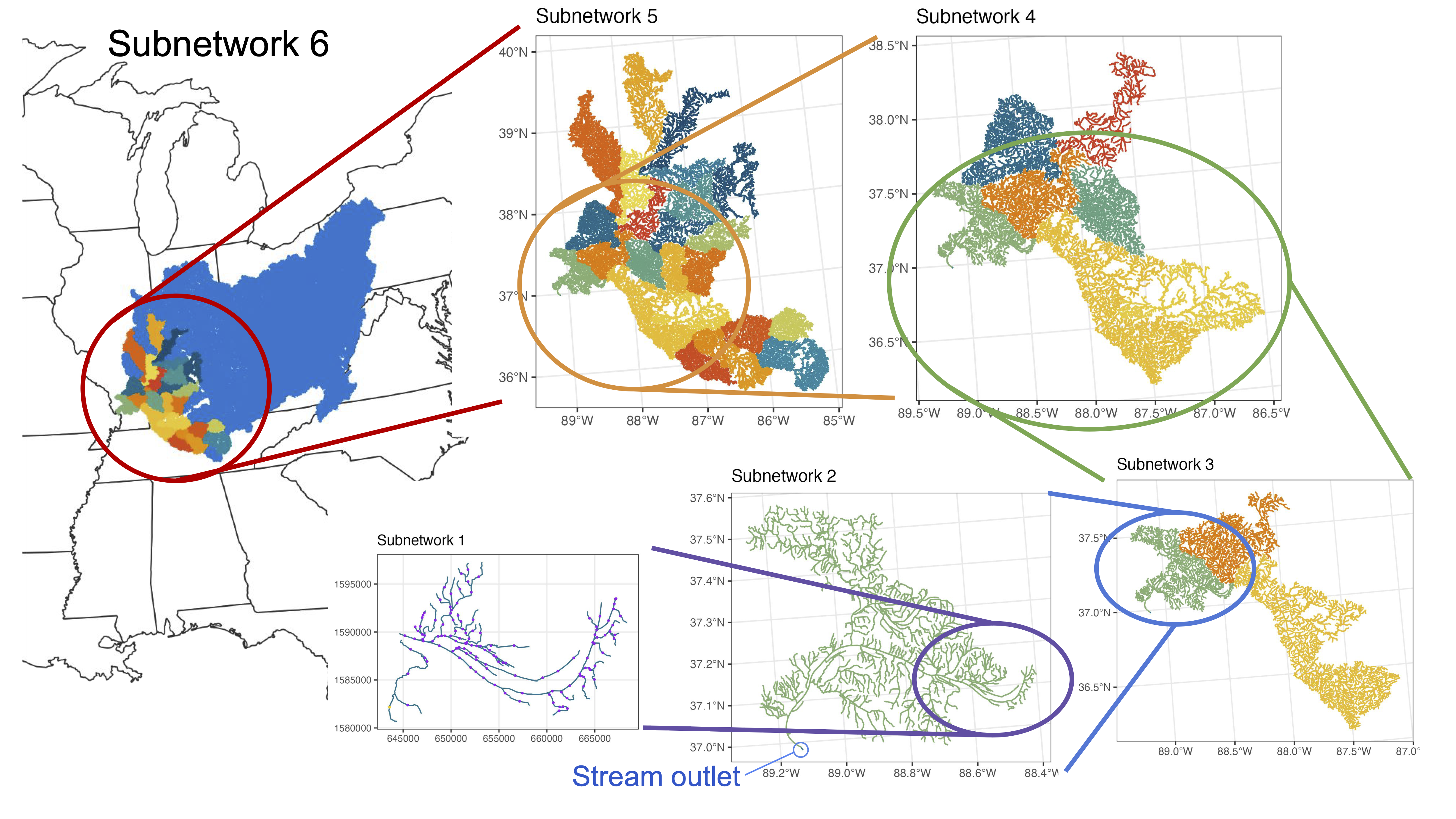
My research:
Making pretty maps, doing analyses
Teaching materials (these slides and the website are made with Quarto!)
Syllabus and course goals
The syllabus (as well as lots of other information) can be found on our course website
Feel free to follow along online as I run through the syllabus!
This course is intended to give students a foundational understanding of programming in the statistical language R. This knowledge is intended to be broadly useful wherever you encounter data in your education and career. General topics we will focus on include:
Developing intermediate data management and visualization skills
Organizing projects and creating reproducible research
Cleaning data
Linking multiple data sets together
Learning basic programming skills
By the end of this course you should feel confident approaching any data you encounter in the future. We will cover almost no statistics, however it is the intention that this course will leave you prepared to progress in CS&SS or STAT courses with the ability to focus on statistics instead of coding. Additionally, the basic concepts you learn will be applicable to other programming languages and research in general, such as logic and algorithmic thinking.
Logistics: General
Lecture: Tuesdays 4:30-6:20pm, Thomson Hall Room 325
Office Hours: Wednesdays 4-6pm, Savery Hall Room 117 (CSSCR Lab)
How to Contact Me
Please post your questions on Ed Discussion (accessible through Canvas) rather than emailing me. This helps ensure I won’t miss them!
Logistics: Three Tools for Class
Communication
Learning is collaborative! In addition to being the place to communicate with me, please use Ed Discussion to ask each other questions, share resources, etc.
Homework & Peer-Reviews
We will be using Canvas only for homework & peer review submissions and to house lecture recordings and Zoom links.
Course Content
All course content (lecture slides and homework instructions) will be accessible on our course website.
Prerequisites
None 😎
Computers
I recommend bringing a laptop to class so you can follow along and practice during class.
Keep In Mind
The versions of R, RStudio, and Quarto (as well as any packages you have installed) will not necessarily be the same/up to date if you do your work on different computers. My advice is to consistently use the same device for homework assignments or to make sure to download the latest versions of R, RStudio, and Quarto when using a new machine.
Readings
Textbooks: This course has no textbook. However, I will be suggesting selections from R for Data Science to pair with each week’s topic. While not required, I strongly suggest reading those selections before doing the homework for that week.
Course Assessment
Final grade
Credit/No Credit (C/NC); You need at least 60% to get Credit
Homework (75%; assessed by peers)
9 total homeworks; assessed on a 0-3 point rubric. Assigned at the end of lecture sessions and due a week later.
Evaluation
Points
Not submitted.
0
Turned in but low effort, ignoring many directions.
1
Decent effort, followed directions with some minor issues.
2
Submitted
3
Peer Grading (25%; assessed by me)
One per homework, assessed on a binary satisfactory/unsatisfactory scale. Due 5 days after homework due date.
Evaluation
Points
Didn’t follow all peer-review instructions.
0
Peer review is at least several sentences long, mentions any and all key issues from the assignment, and points out at least one positive thing in your peer’s work (and hopefully more!).
1
Due Dates and Late Policy
Homework/peer grading instructions and deadlines can be found on the Homework page of the course website. All homework will be turned in on Canvas by 4:30pm the day it is due.
No late assignments will be accepted to ensure you receive feedback at regular intervals and stay on track. The grading is lenient, so submit whatever you have by each deadline, and your grade will be fine if you miss submitting an assignment or two due to illness or emergencies.
Peer reviews are randomly assigned when the due date/time is reached. Therefore, if you don’t submit your homework, you will not be given a peer’s homework to review and vice versa.
Ugh, peer grading?
Yes, because:
You will write your reports better knowing others will see them
You learn alternative approaches to the same problem
You will have more opportunities to practice and have the material sink in
How to peer review:
Leave constructive comments: You’ll only get the point if you write at least several sentences that includes
Any key issues from the assignment and,
Points out something positive in your peer’s work.
Send me a private message on Ed Discussion if you would like your assignment to be regraded or for me to provide feedback if no peer review was given.
Academic Integrity
Academic integrity is essential to this course and to your learning. Violations of the academic integrity policy include but are not limited to:
Copying from a peer
Copying from an online resource
Using resources from a previous iteration of the course.
I hope you will collaborate with peers on assignments and use Internet resources when questions arise to help solve issues. The key is that you ultimately submit your own work.
Anything found in violation of this policy will be automatically given a score of 0 with no exceptions. If the situation merits, it will also be reported to the UW Student Conduct Office, at which point it is out of my hands. If you have any questions about this policy, please do not hesitate to reach out and ask.
Classroom Environment
I’m committed to fostering a friendly and inclusive classroom environment in which all students have an equal opportunity to learn and succeed. This course is an attempt to make an often difficult and frustrating experience (learning R for the first time) less obfuscating, daunting, and stressful. That said, learning happens in different ways at at a different pace for everyone. Learning is also a collaborative and creative process and my aim is to create an environment in which you all feel comfortable asking questions of me and each other. Treat your peers and yourself with empathy and respect as you all approach this topic from a range of backgrounds and experiences (in programming and in life).
Classroom Environment…
Names & Pronouns: Everyone deserves to be addressed respectfully and correctly. You are welcome to send me your preferred name and correct gender pronouns at any time.
Diversity: Diverse backgrounds, embodiments, and experiences are essential to the critical thinking endeavor at the heart of university education. Therefore, I expect you to follow the UW Student Conduct Code in your interactions with your colleagues and me in this course by respecting the many social and cultural differences among us, which may include, but are not limited to: age, cultural background, disability, ethnicity, family status, gender identity and presentation, body size/shape, citizenship and immigration status, national origin, race, religious and political beliefs, sex, sexual orientation, socioeconomic status, and veteran status.
Accommodations
Accessibility & Accommodations: Your experience in this class is important to me. If you have already established accommodations with Disability Resources for Students (DRS), please communicate your approved accommodations to me at your earliest convenience so we can discuss your needs in this course. If you have not yet established services through DRS, but have a temporary health condition or permanent disability that requires accommodations (conditions include but not limited to; mental health, attention-related, learning, vision, hearing, physical or health impacts), you are welcome to contact DRS at 206-543-8924, uwdrs@uw.edu, or through their website.
Religious Accommodations: Washington state law requires that UW develop a policy for accommodation of student absences or significant hardship due to reasons of faith or conscience, or for organized religious activities. The UW's policy, including more information about how to request an accommodation, is available at Religious Accommodations Policy. Accommodations must be requested within the first two weeks of this course using the Religious Accommodations Request form.
Help and Feedback
Getting Help: If at any point during the quarter you find yourself struggling to keep up, please let me know! I am here to help. A great place to start this process is by chatting before or after class, attending office hours, and/or reaching out on Ed Discussion. As much as possible, I encourage you to use my office hours.
Also, help one another as you navigate this course! Use Ed Discussion to discuss questions with each other, and feel free to form study/practice groups.
Feedback
If you have feedback on any part of this course or the classroom environment I want to hear it! You can submit anonymous feedback here. I will also send out a mid-quarter feedback survey.
Asking Questions
Don’t ask like this:
tried lm(y~x) but it iddn’t work wat do
Instead, ask like this:
y <- seq(1:10) + rnorm(10)
x <- seq(0:10)
model <- lm(y ~ x)
Running the block above gives me the following error, anyone know why?
Error in model.frame.default(formula = y ~ x,
drop.unused.levels = TRUE) : variable lengths differ
(found for 'x')
FYI
If you ask me a question directly on Ed Discussion or in office hours, I may send out your question (anonymously) along with my answer to the whole course.
Questions?
Introduction to R, RStudio, and Quarto
A Note on Slide Formatting
Bold usually indicates an important vocabulary term. Remember these!
Italics indicate emphasis but also are used to point out things you must click with a mouse.
For example: “Please click File > Print”
Code represents R code or keyboard shortcuts you can use to perform actions.
For example: “Press Ctrl-P to open the print dialogue.”
Code chunks that span the page represent actual R code embedded in the slides.
7*49
A Note on Slide Formatting
Bold usually indicates an important vocabulary term. Remember these!
Italics indicate emphasis but also are used to point out things you must click with a mouse.
For example: “Please click File > Print”
Code represents R code you could use to perform actions.
For example: “Press Ctrl-P to open the print dialogue.”
Code chunks that span the page represent actual R code embedded in the slides.
7*49# Sometimes important stuff is highlighted!
A Note on How to Use These Slides
Since the lectures for this class were created using Quarto, there are numerous built-in features meant to facilitate your learning, particularly of R.
The bars in the bottom left-hand corner will show you a table of contents for the entire slideshow, allowing you to find what you’re looking for more easily.
If you hover over any chunk of R code embedded in the slides you will see a clipboard which you can click to copy the code. You can then paste it in your own Quarto document or R script to run it in your session of RStudio.
To get a PDF version of these slides click File > Print from your internet browser, select Save as PDF as the Destination or Printer, and make sure the Layout is set to Landscape. (Note: the PDF Export Mode in Tools actually cuts off content which is why I’m not recommending it)
Clicking on the paintbrush in the bottom left-hand corner allows you to draw directly on the slides, in a very Microsoft Paint kind of way. See if it’s useful but I make no promises!
Type ? at any time to see all the available key-board shortcuts.
Some pages are scrollable.
Why R?
R is a programming language built for statistical computing.
If one already knows Stata or similar software, why use R?
R is free.
R has a very large community.
R can handle virtually any data format.
R makes replication easy.
R is a language so it can do everything.
R skills transfer to other languages like Python and Julia.
R Studio
R Studio is a “front-end” or integrated development environment (IDE) for R that can make your life easier.
We’ll show RStudio can…
Organize your code, output, and plots
Auto-complete code and highlight syntax
Help view data and objects
Enable easy integration of R code into documents with Quarto
It can also…
Manage git repositories (version control)
Run interactive tutorials
Handle other languages like C++, Python, SQL, HTML, and shell scripting
Selling You on Quarto
Built upon many of the developments of the R Markdown ecosystem, Quarto distills them into one coherent system and additionally expands its functionality by supporting other programming languages besides R, including Python and Julia.
Selling You on Quarto
The ability to create Quarto files in R is a powerful advantage. It allows us to:
Document analyses by combining text, code, and output
Works with LaTeX and HTML for math and more formatting control
Downloading R and RStudio
If you don’t already have R and RStudio on your machine, now is the time to do so! Follow the instructions in the syllabus.
Getting Started
Open up RStudio now and choose File > New File > R Script.
Then, let’s get oriented with the interface:
Top Left: Code editor pane, data viewer (browse with tabs)
Bottom Left: Console for running code (> prompt)
Top Right: List of objects in environment, code history tab.
Bottom Right: Tabs for browsing files, viewing plots, managing packages, and viewing help files.
Editing and Running Code
There are several ways to run R code in RStudio:
Highlight lines in the editor window and click Run at the top right corner of said window or hit Ctrl+Enter or ⌘+Enter to run them all.
Editing and Running Code
There are several ways to run R code in RStudio:
Highlight lines in the editor window and click Run at the top right corner of said window or hit Ctrl+Enter or ⌘+Enter to run them all.
With your caret1 on a line you want to run, hit Ctrl+Enter or ⌘+Enter. Note your caret moves to the next line, so you can run code sequentially with repeated presses.
Type individual lines in the console and press Enter.
In quarto documents, click within a code chunk and click the green arrow to run the chunk. The button beside that () runs all prior chunks.
The console will show the lines you ran followed by any printed output.
Incomplete Code
If you mess up (e.g. leave off a parenthesis), R might show a + sign prompting you to finish the command:
> (11-2+
Finish the command or hit Esc to get out of this.
R as a Calculator
In the console, type 123 + 456 + 789 and hit Enter.
123+456+789
[1] 1368
The [1] in the output indicates the numeric index of the first element on that line.
Now in your blank R document in the editor, try typing the line sqrt(400) and either clicking Run or hitting Ctrl+Enter or ⌘+Enter.
Functions can have a wide range of arguments and some are required for the function to run, while others remain optional. You can see from each functions’ help page which are not required because they will have an = with some default value pre-selected. If there is no = it is up to the user to define that value and it’s therefore a required specification.
Help
If we didn’t have a good guess as to what sqrt() will do, we can type ?sqrt in the console and look at the Help panel on the bottom right.
?sqrt
If you’re trying to look up the help page for a function and can’t remember its name you can search by a keyword and you will get a list of help pages containing said keyword.
??exponential
Help
Help files provide documentation on how to use functions and what functions produce. They will generally consist of the following sections:
Description - What does it do?
Usage - How do you write it?
Arguments - What arguments does it take; which are required; what are the defaults?
Details - A more in-depth description
Value - What does the function return?
See Also - Related R functions
Examples - Example (& reproducible) code
Objects
R stores everything as an object, including data, functions, models, and output.
Creating an object can be done using the assignment operators<- or =: . . .
new.object <-144x =5
Operators like <- are functions that look like symbols but typically sit between their arguments (e.g. numbers or objects) instead of having them inside () like in sqrt(x).
We do math with operators, e.g., x + y.
+ is the addition operator!
Calling Objects
You can display or “call” an object simply by using its name.
new.object
[1] 144
Naming Objects
Object names must begin with a letter and can contain letters, numbers, ., and _.
Try to be consistent in naming objects. RStudio auto-complete means long, descriptive names are better than short, vague ones! Good names save confusion later!
snake_case, where you separate lowercase words with _ is a common and practical naming convention that I strongly recommend.
An object’s name represents the information stored in that object, so you can treat the object’s name as if it were the values stored inside. . . .
new.object +10
[1] 154
new.object + new.object
[1] 288
sqrt(new.object)
[1] 12
Comments
Anything written after #1 will be ignored by R.
# create vector of ages of studentsages <-c(45, 21, 27, 34, 23, 24, 24)# get average age of studentsmean(ages)
[1] 28.28571
Comments help collaborators and future-you understand what, and more importantly, why you are doing what you’re doing with that specific line/chunk of code.
Additionally, comments allow you to explain your overall coding plan and record anything important that you’ve discovered along the way.
Vectors
A vector is one of many data types available in R. Specifically, it is a series of elements, such as numbers, strings, or booleans (i.e. TRUE, FALSE).
You can create a vector using the function c() which stands for “combine” or “concatenate”. . . .
new.object <-c(4, 9, 16, 25, 36)new.object
[1] 4 9 16 25 36
If you name an object the same name as an existing object, it will overwrite it.
You can provide a vector as an argument for many functions. . . .
sqrt(new.object)
[1] 2 3 4 5 6
More Complex Objects
There are other, more complex data types in R which we will discuss later in the quarter! These include matrices, arrays, lists, and dataframes.
Most data sets you will work with will be read into R and stored as a dataframe, so this course will mainly focus on manipulating and visualizing these objects.
Quarto
Creating a Quarto Document
Let’s try making an Quarto file:
Choose File > New File > Quarto Document…
Make sure HTML Output is selected
In the Title box call this test document “My First Qmd” and click Create
Save this document somewhere (you can delete it later) (either with File > Save or clicking towards the top left of the source pane).
Lastly, click Render at the top of the source pan to “knit” your document into an html file. This will produce a minimal webpage since we only have a title. We need to add more content!
If you want to create PDF output in the future, you’ll need to run the following code in your console.
---
title: "ggplot2 demo"
author: "Norah Jones"
date: "5/22/2021"
format:
  html:
    fig-width: 8
    fig-height: 4
    code-fold: true
---

## Air Quality

@fig-airquality further explores the impact of temperature on ozone level.

```{r}
#| label: fig-airquality
#| fig-cap: "Temperature and ozone level."
#| warning: false

library(ggplot2)
ggplot(airquality, aes(Temp, Ozone)) +
  geom_point() +
  geom_smooth(method = "loess")
```
The rendered output of the qmd file shown on the previous tab.
Elements of a Quarto document include:
An (optional) YAML header (surrounded by ---s).
Plain text and any associated formatting.
Chunks of code (surrounded by ``` s) and/or their output.
Quarto Headers
The header of a .qmd file is a YAML1code block, and everything else is part of the main document. Try adding some of these other fields to your YAML and re-render it to see what it looks like.
**bold/strong emphasis***italic/normal emphasis*# Header## Subheader### Subsubheader> Block quote from> famous person
Quarto Syntax Continued
This is all basic markdown syntax which you can learn about here.
Output
Ordered lists
Are real easy
Even with sublists
Or with lazy numbering
Unordered lists
Are also real easy
Also even with sublists
And subsublists
Syntax
1. Ordered lists1. Are real easy1. Even with sublists1. Or with lazy numbering* Unordered lists* Are also real easy+ Also even with sublists- And subsublists
Formulae and Syntax
Output
Include math \(y= \left( \frac{2}{3} \right)^2\) inline.
Or centered on your page like so:
\[\frac{1}{n} \sum_{i=1}^{n} x_i = \bar{x}_n\]
Or write code-looking font.
Or a block of code:
y<-1:5z<-y^2
Syntax
Include math $y= \left(\frac{2}{3} \right)^2$ inline. Or centered on your page like so: $$\frac{1}{n} \sum_{i=1}^{n}x_i = \bar{x}_n$$Or write`code-looking font`.Or a block of code:```{r squared}y <- 1:5z <- y^2```
Quarto Tinkering
Quarto docs can be modified in many ways. Visit these links for more information.
Inside Quarto, lines of R code are called chunks. Code is sandwiched between sets of three backticks and {r}. This chunk of code…
```{r cars}summary(cars)```
Produces this output in your document:
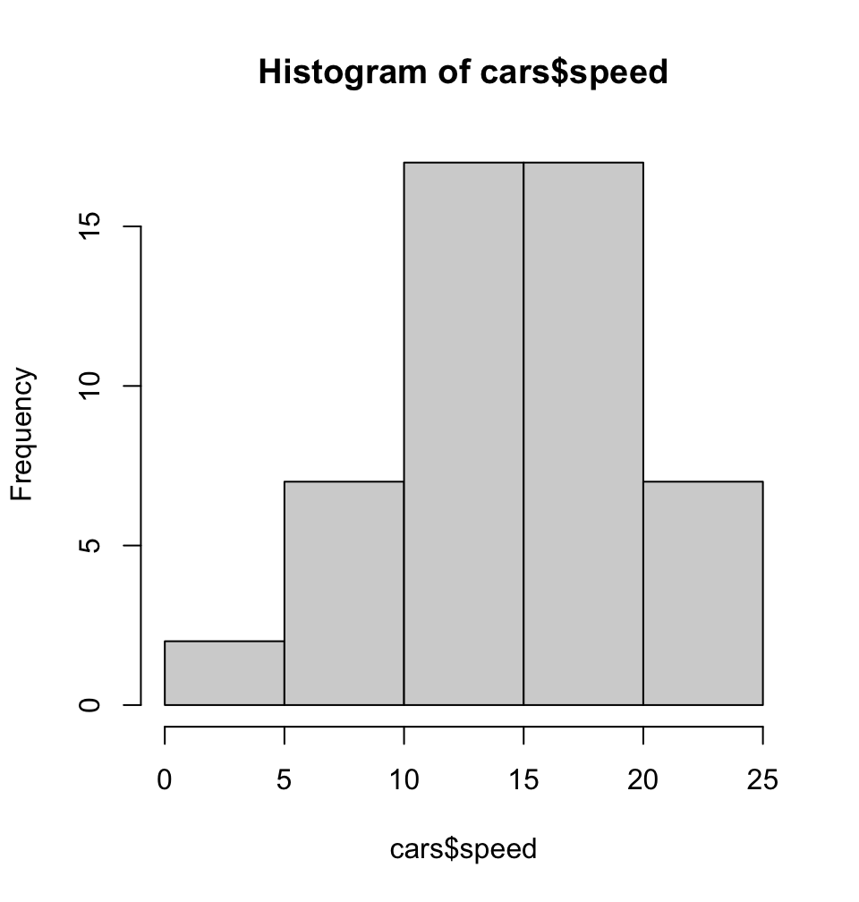
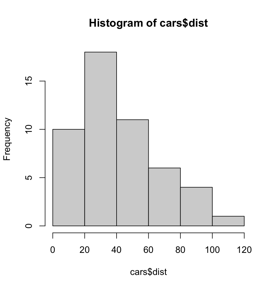
summary(cars)
     speed           dist
 Min.   : 4.0   Min.   :  2.00
 1st Qu.:12.0   1st Qu.: 26.00
 Median :15.0   Median : 36.00
 Mean   :15.4   Mean   : 42.98
 3rd Qu.:19.0   3rd Qu.: 56.00
 Max.   :25.0   Max.   :120.00
Add this code chunk to your document!
Chunk Options
Chunks have options that control what happens with their code. They are specified as special comments at the top of a block. For example:
```{r barchart}#| label: bar-chart#| eval: false#| fig-cap: "A line plot on a polar axis"```
Chunk Options
Some useful and common options include:
echo: false - Keeps R code from being shown in the document
eval: false - Shows R code in the document without running it
include: false - Hides all output but still runs code (good for setup chunks where you load packages!)
output: false - Doesn’t include the results of that code chunk in the output
cache: true - Saves results of running that chunk so if it takes a while, you won’t have to re-run it each time you re-render the document
fig.height: 5, fig.width: 5 - modify the dimensions of any plots that are generated in the chunk (units are in inches)
fig.cap: "Text" - add a caption to your figure in the chunk
Playing with Chunk Options
Try adding or changing the chunk options for the chunk in my_first_Rmd.qmd and re-render your document to see what happens.
```{r fenced}#| eval: falsesummary(cars)```
In-Line R code
Sometimes we want to insert a value directly into our text. We do that using code in single backticks starting off with r.
Four score and seven years ago is the same as `r 4*20 + 7` years.
Four score and seven years ago is the same as 87 years.
Maybe we’ve saved a variable in a code chunk that we want to reference in the text:
x <-sqrt(77)
The value of `x` rounded to the nearest two decimals is `r round(x, 2)`.
The value of x rounded to the nearest two decimals is 8.77.
This is Amazing!
Having R dump values directly into your document protects you from silly mistakes:
Never wonder “how did I come up with this quantity?” ever again: Just look at your formula in your .qmd file!
Consistency! No “find/replace” mishaps; reference a variable in-line throughout your document without manually updating if the calculation changes (e.g. reporting sample sizes).
You are more likely to make a typo in a “hard-coded” number than you are to write R code that somehow runs but gives you the wrong thing.
Example: Keeping Dates
In your YAML header, make the date come from R’s Sys.time() function by changing:
date: "March 26, 2024"
to
date: "`r Sys.time()`"
Base R and Packages
Base R
Simply by downloading R you have access to what is referred to as Base R. That is, the built-in functions and datasets that R comes equipped with, right out of the box.
Examples that we’ve already seen include <-, sqrt(), +, Sys.time(), and summary() but there are obviously many many more.
You can see a whole list of what Base R contains by running library(help = "base") in the console.
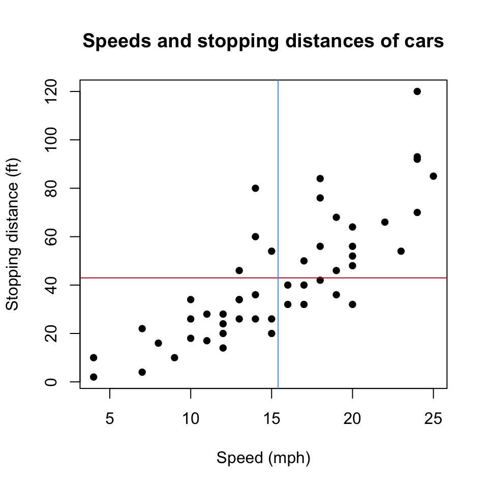
A Base R Dataset: cars
In the sample Quarto document you are working on, we can load the built-in data cars, which loads as a dataframe, a type of object mentioned earlier. Then, we can look at it in a couple different ways.
data(cars) loads this dataframe into the Global Environment.
View(cars) pops up a Viewer tab in the source pane (“interactive” use only, don’t put in Quarto document!).
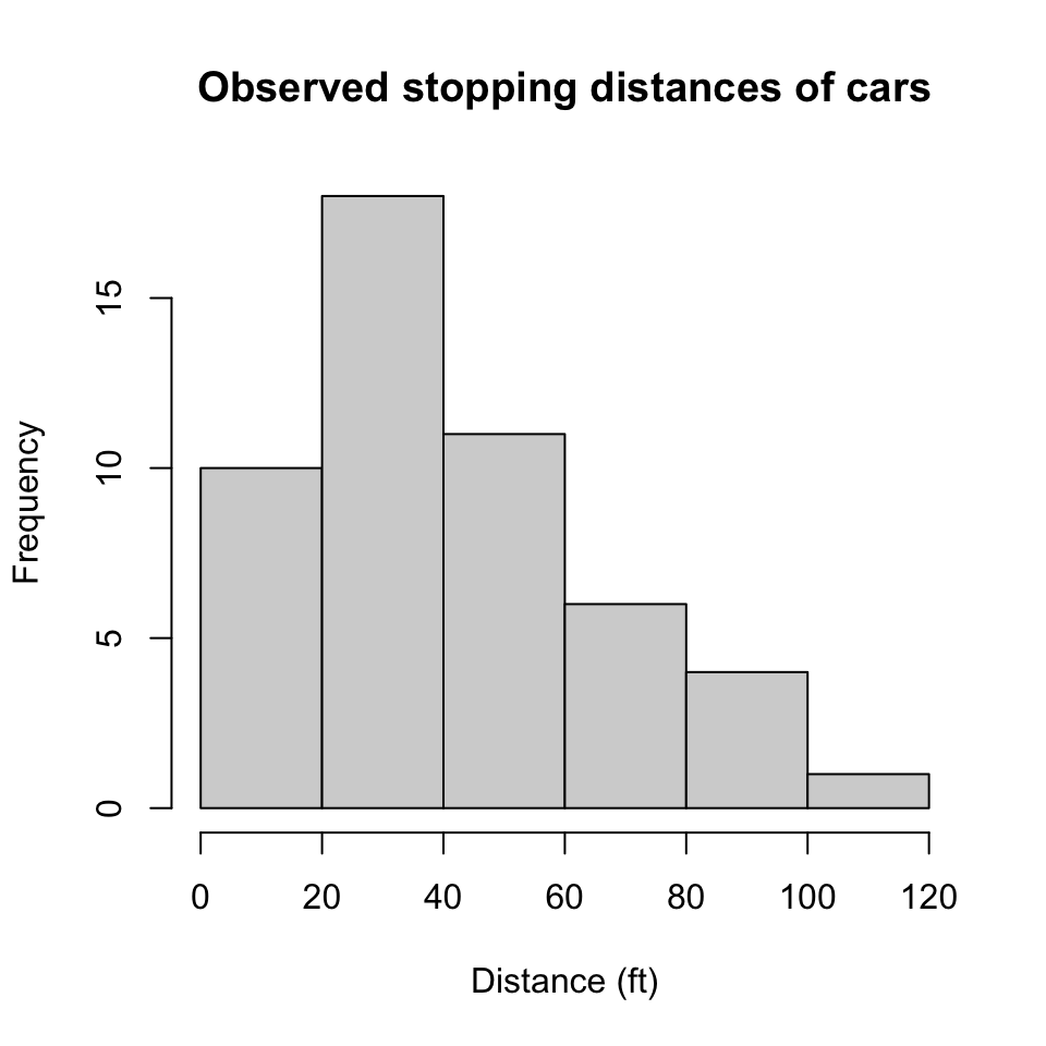
head(cars, 5) # prints first 5 rows, can use tail() too
plot(dist ~ speed, data = cars,xlab ="Speed (mph)",ylab ="Stopping distance (ft)",main ="Speeds and stopping distances of cars",pch =16) # Point shapeabline(h =mean(cars$dist), col ="firebrick") # add horizontal line (y-value)abline(v =mean(cars$speed), col ="cornflowerblue") # add vertical line (x-value)
Note
dist ~ speed is a formula of the type y ~ x. The first element (dist) gets plotted on the y-axis and the second (speed) goes on the x-axis. Regression formulae follow this convention as well!
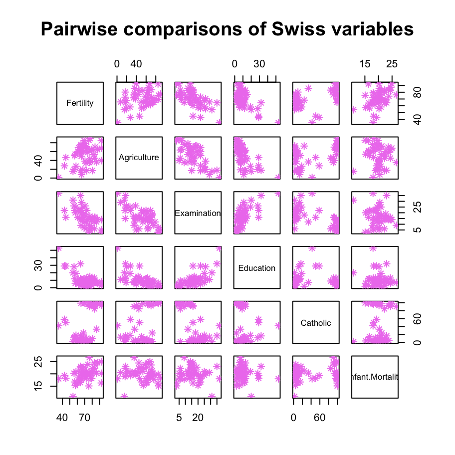
Base R is pretty…Basic
We can also make scatterplots to show the relationship between two variables.
pairs(swiss, pch =8, col ="violet",main ="Pairwise comparisons of Swiss variables")
Packages
What makes R so powerful though is it’s extensive library of packages. Due to it’s open-source nature, anyone (even you!) can write a package that others can use.
Packages contain pre-made functions and/or data that can be used to extend Base R’s capabilities.
Base R/Package Analogy
Base R is like creating a recipe from scratch: going to the store and buying all the ingredients and cooking it by yourself. Using a package is more akin to using a meal-kit service: you still have to cook but you’re provided with the ingredients and step-by-step instructions for making the recipe.
This downloads the package to your local machine (or the server of whatever remote machine you’re using). Thus, you only every need to do it once for each package2!
Installing Packages
To use a package outside of Base R you need to do two things:
Download the package from CRAN (The Comprehensive RArchive Network) by running the following in your console1:
This downloads the package to your local machine (or the server of whatever remote machine you’re using). Thus, you only every need to do it once for each package2!
Once a package is installed, you need to load it into the current session of R so you can use it. You’ll do this by putting the following in an R Script or embedded in a code chunk in a Quarto file:
library(package_name)
gt Package
Let’s make a table that’s more polished than the code-y output R automatically gives us. To do this, we’ll want to install our first package called gt. In the console, run: install.packages("gt").
Different Syntax
Notice that unlike the library() command, the name of a package to be installed must be in quotes? This is because the name here is a search term (text, not an object!) while for library() it is an actual R object.
library(gt) # loads gt, do once in your sessiongt(as.data.frame.matrix(summary(swiss)))
Nesting Functions
Note that we put the summary(swiss) function call inside the as.data.frame.matrix() call which all went into the gt() function. This is called nesting functions and is very common. I’ll introduce a method next week to avoid confusion from nesting too many functions inside each other.
gt() takes as its first argument a data.frame-type object, while summary() produces a table-type object. Therefore, as.data.frame.matrix() was additionally needed to turn the table into a data.frame.
We no longer need as.data.frame.matrix() since we’re no longer using summary(). Both head() and gt_preview() take a data.frame-type object as their first argument which is the same data type as swiss.
 Run at the top right corner of said window or hit
  to run the chunk. The button beside that (
 ) runs all prior chunks.
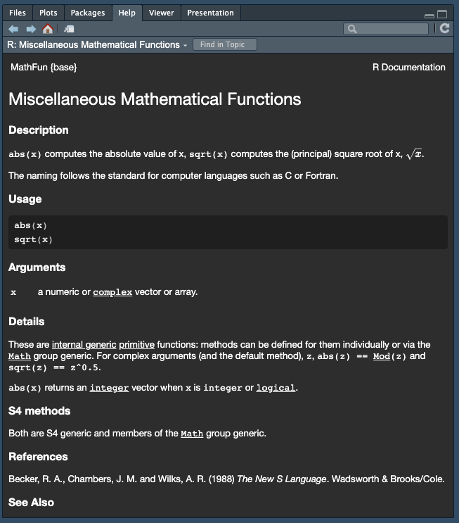
 towards the top left of the source pane).
 Render at the top of the source pan to “knit” your document into an html file. This will produce a minimal webpage since we only have a title. We need to add more content!
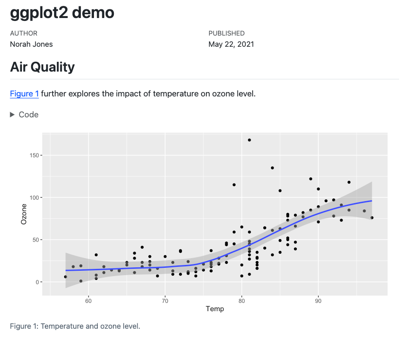

Comments
Anything written after
#1 will be ignored by R.Comments help collaborators and future-you understand what, and more importantly, why you are doing what you’re doing with that specific line/chunk of code.
Additionally, comments allow you to explain your overall coding plan and record anything important that you’ve discovered along the way.